
\[\newcommand{\norm}[1]{\lVert#1\rVert} \renewcommand{\top}{\mathsf{T}} \newcommand{\SQ}{\mathrm{SQ}}\]
2クラス問題に対する量子インスパイアード古典アルゴリズム#
このノートブックでは,2クラス問題について考察します.具体的にはIRISデータセットを例にして,線形識別関数の係数ベクトル\(\theta\)に関する\(\SQ(\theta)\)を考察します.そして,テスト用のデータがどちらのクラスであるかどうか,\(\theta\)をそのまま構成することなく,判別することについて考えます.
[1]:
import numpy as np
import scipy as sp
import numpy.linalg as la
import random
import cmath, math
import matplotlib.pyplot as plt
import pprint
from sklearn.datasets import load_iris
from sklearn.model_selection import train_test_split
データセットを読み込む#
IRISデータセットはPythonのライブラリscikit-learnに含まれています. このライブラリにあるload_irisを使うことで読み込むことができます.次のセルでデータをロードしてみます.
[2]:
from sklearn.datasets import load_iris
iris = load_iris()
pprint.pprint(iris)
{'DESCR': '.. _iris_dataset:\n'
          '\n'
          'Iris plants dataset\n'
          '--------------------\n'
          '\n'
          '**Data Set Characteristics:**\n'
          '\n'
          '    :Number of Instances: 150 (50 in each of three classes)\n'
          '    :Number of Attributes: 4 numeric, predictive attributes and the '
          'class\n'
          '    :Attribute Information:\n'
          '        - sepal length in cm\n'
          '        - sepal width in cm\n'
          '        - petal length in cm\n'
          '        - petal width in cm\n'
          '        - class:\n'
          '                - Iris-Setosa\n'
          '                - Iris-Versicolour\n'
          '                - Iris-Virginica\n'
          '                \n'
          '    :Summary Statistics:\n'
          '\n'
          '    ============== ==== ==== ======= ===== ====================\n'
          '                    Min  Max   Mean    SD   Class Correlation\n'
          '    ============== ==== ==== ======= ===== ====================\n'
          '    sepal length:   4.3  7.9   5.84   0.83    0.7826\n'
          '    sepal width:    2.0  4.4   3.05   0.43   -0.4194\n'
          '    petal length:   1.0  6.9   3.76   1.76    0.9490  (high!)\n'
          '    petal width:    0.1  2.5   1.20   0.76    0.9565  (high!)\n'
          '    ============== ==== ==== ======= ===== ====================\n'
          '\n'
          '    :Missing Attribute Values: None\n'
          '    :Class Distribution: 33.3% for each of 3 classes.\n'
          '    :Creator: R.A. Fisher\n'
          '    :Donor: Michael Marshall (MARSHALL%PLU@io.arc.nasa.gov)\n'
          '    :Date: July, 1988\n'
          '\n'
          'The famous Iris database, first used by Sir R.A. Fisher. The '
          'dataset is taken\n'
          "from Fisher's paper. Note that it's the same as in R, but not as in "
          'the UCI\n'
          'Machine Learning Repository, which has two wrong data points.\n'
          '\n'
          'This is perhaps the best known database to be found in the\n'
          "pattern recognition literature.  Fisher's paper is a classic in the "
          'field and\n'
          'is referenced frequently to this day.  (See Duda & Hart, for '
          'example.)  The\n'
          'data set contains 3 classes of 50 instances each, where each class '
          'refers to a\n'
          'type of iris plant.  One class is linearly separable from the other '
          '2; the\n'
          'latter are NOT linearly separable from each other.\n'
          '\n'
          '.. topic:: References\n'
          '\n'
          '   - Fisher, R.A. "The use of multiple measurements in taxonomic '
          'problems"\n'
          '     Annual Eugenics, 7, Part II, 179-188 (1936); also in '
          '"Contributions to\n'
          '     Mathematical Statistics" (John Wiley, NY, 1950).\n'
          '   - Duda, R.O., & Hart, P.E. (1973) Pattern Classification and '
          'Scene Analysis.\n'
          '     (Q327.D83) John Wiley & Sons.  ISBN 0-471-22361-1.  See page '
          '218.\n'
          '   - Dasarathy, B.V. (1980) "Nosing Around the Neighborhood: A New '
          'System\n'
          '     Structure and Classification Rule for Recognition in Partially '
          'Exposed\n'
          '     Environments".  IEEE Transactions on Pattern Analysis and '
          'Machine\n'
          '     Intelligence, Vol. PAMI-2, No. 1, 67-71.\n'
          '   - Gates, G.W. (1972) "The Reduced Nearest Neighbor Rule".  IEEE '
          'Transactions\n'
          '     on Information Theory, May 1972, 431-433.\n'
          '   - See also: 1988 MLC Proceedings, 54-64.  Cheeseman et al"s '
          'AUTOCLASS II\n'
          '     conceptual clustering system finds 3 classes in the data.\n'
          '   - Many, many more ...',
 'data': array([[5.1, 3.5, 1.4, 0.2],
       [4.9, 3. , 1.4, 0.2],
       [4.7, 3.2, 1.3, 0.2],
       [4.6, 3.1, 1.5, 0.2],
       [5. , 3.6, 1.4, 0.2],
       [5.4, 3.9, 1.7, 0.4],
       [4.6, 3.4, 1.4, 0.3],
       [5. , 3.4, 1.5, 0.2],
       [4.4, 2.9, 1.4, 0.2],
       [4.9, 3.1, 1.5, 0.1],
       [5.4, 3.7, 1.5, 0.2],
       [4.8, 3.4, 1.6, 0.2],
       [4.8, 3. , 1.4, 0.1],
       [4.3, 3. , 1.1, 0.1],
       [5.8, 4. , 1.2, 0.2],
       [5.7, 4.4, 1.5, 0.4],
       [5.4, 3.9, 1.3, 0.4],
       [5.1, 3.5, 1.4, 0.3],
       [5.7, 3.8, 1.7, 0.3],
       [5.1, 3.8, 1.5, 0.3],
       [5.4, 3.4, 1.7, 0.2],
       [5.1, 3.7, 1.5, 0.4],
       [4.6, 3.6, 1. , 0.2],
       [5.1, 3.3, 1.7, 0.5],
       [4.8, 3.4, 1.9, 0.2],
       [5. , 3. , 1.6, 0.2],
       [5. , 3.4, 1.6, 0.4],
       [5.2, 3.5, 1.5, 0.2],
       [5.2, 3.4, 1.4, 0.2],
       [4.7, 3.2, 1.6, 0.2],
       [4.8, 3.1, 1.6, 0.2],
       [5.4, 3.4, 1.5, 0.4],
       [5.2, 4.1, 1.5, 0.1],
       [5.5, 4.2, 1.4, 0.2],
       [4.9, 3.1, 1.5, 0.2],
       [5. , 3.2, 1.2, 0.2],
       [5.5, 3.5, 1.3, 0.2],
       [4.9, 3.6, 1.4, 0.1],
       [4.4, 3. , 1.3, 0.2],
       [5.1, 3.4, 1.5, 0.2],
       [5. , 3.5, 1.3, 0.3],
       [4.5, 2.3, 1.3, 0.3],
       [4.4, 3.2, 1.3, 0.2],
       [5. , 3.5, 1.6, 0.6],
       [5.1, 3.8, 1.9, 0.4],
       [4.8, 3. , 1.4, 0.3],
       [5.1, 3.8, 1.6, 0.2],
       [4.6, 3.2, 1.4, 0.2],
       [5.3, 3.7, 1.5, 0.2],
       [5. , 3.3, 1.4, 0.2],
       [7. , 3.2, 4.7, 1.4],
       [6.4, 3.2, 4.5, 1.5],
       [6.9, 3.1, 4.9, 1.5],
       [5.5, 2.3, 4. , 1.3],
       [6.5, 2.8, 4.6, 1.5],
       [5.7, 2.8, 4.5, 1.3],
       [6.3, 3.3, 4.7, 1.6],
       [4.9, 2.4, 3.3, 1. ],
       [6.6, 2.9, 4.6, 1.3],
       [5.2, 2.7, 3.9, 1.4],
       [5. , 2. , 3.5, 1. ],
       [5.9, 3. , 4.2, 1.5],
       [6. , 2.2, 4. , 1. ],
       [6.1, 2.9, 4.7, 1.4],
       [5.6, 2.9, 3.6, 1.3],
       [6.7, 3.1, 4.4, 1.4],
       [5.6, 3. , 4.5, 1.5],
       [5.8, 2.7, 4.1, 1. ],
       [6.2, 2.2, 4.5, 1.5],
       [5.6, 2.5, 3.9, 1.1],
       [5.9, 3.2, 4.8, 1.8],
       [6.1, 2.8, 4. , 1.3],
       [6.3, 2.5, 4.9, 1.5],
       [6.1, 2.8, 4.7, 1.2],
       [6.4, 2.9, 4.3, 1.3],
       [6.6, 3. , 4.4, 1.4],
       [6.8, 2.8, 4.8, 1.4],
       [6.7, 3. , 5. , 1.7],
       [6. , 2.9, 4.5, 1.5],
       [5.7, 2.6, 3.5, 1. ],
       [5.5, 2.4, 3.8, 1.1],
       [5.5, 2.4, 3.7, 1. ],
       [5.8, 2.7, 3.9, 1.2],
       [6. , 2.7, 5.1, 1.6],
       [5.4, 3. , 4.5, 1.5],
       [6. , 3.4, 4.5, 1.6],
       [6.7, 3.1, 4.7, 1.5],
       [6.3, 2.3, 4.4, 1.3],
       [5.6, 3. , 4.1, 1.3],
       [5.5, 2.5, 4. , 1.3],
       [5.5, 2.6, 4.4, 1.2],
       [6.1, 3. , 4.6, 1.4],
       [5.8, 2.6, 4. , 1.2],
       [5. , 2.3, 3.3, 1. ],
       [5.6, 2.7, 4.2, 1.3],
       [5.7, 3. , 4.2, 1.2],
       [5.7, 2.9, 4.2, 1.3],
       [6.2, 2.9, 4.3, 1.3],
       [5.1, 2.5, 3. , 1.1],
       [5.7, 2.8, 4.1, 1.3],
       [6.3, 3.3, 6. , 2.5],
       [5.8, 2.7, 5.1, 1.9],
       [7.1, 3. , 5.9, 2.1],
       [6.3, 2.9, 5.6, 1.8],
       [6.5, 3. , 5.8, 2.2],
       [7.6, 3. , 6.6, 2.1],
       [4.9, 2.5, 4.5, 1.7],
       [7.3, 2.9, 6.3, 1.8],
       [6.7, 2.5, 5.8, 1.8],
       [7.2, 3.6, 6.1, 2.5],
       [6.5, 3.2, 5.1, 2. ],
       [6.4, 2.7, 5.3, 1.9],
       [6.8, 3. , 5.5, 2.1],
       [5.7, 2.5, 5. , 2. ],
       [5.8, 2.8, 5.1, 2.4],
       [6.4, 3.2, 5.3, 2.3],
       [6.5, 3. , 5.5, 1.8],
       [7.7, 3.8, 6.7, 2.2],
       [7.7, 2.6, 6.9, 2.3],
       [6. , 2.2, 5. , 1.5],
       [6.9, 3.2, 5.7, 2.3],
       [5.6, 2.8, 4.9, 2. ],
       [7.7, 2.8, 6.7, 2. ],
       [6.3, 2.7, 4.9, 1.8],
       [6.7, 3.3, 5.7, 2.1],
       [7.2, 3.2, 6. , 1.8],
       [6.2, 2.8, 4.8, 1.8],
       [6.1, 3. , 4.9, 1.8],
       [6.4, 2.8, 5.6, 2.1],
       [7.2, 3. , 5.8, 1.6],
       [7.4, 2.8, 6.1, 1.9],
       [7.9, 3.8, 6.4, 2. ],
       [6.4, 2.8, 5.6, 2.2],
       [6.3, 2.8, 5.1, 1.5],
       [6.1, 2.6, 5.6, 1.4],
       [7.7, 3. , 6.1, 2.3],
       [6.3, 3.4, 5.6, 2.4],
       [6.4, 3.1, 5.5, 1.8],
       [6. , 3. , 4.8, 1.8],
       [6.9, 3.1, 5.4, 2.1],
       [6.7, 3.1, 5.6, 2.4],
       [6.9, 3.1, 5.1, 2.3],
       [5.8, 2.7, 5.1, 1.9],
       [6.8, 3.2, 5.9, 2.3],
       [6.7, 3.3, 5.7, 2.5],
       [6.7, 3. , 5.2, 2.3],
       [6.3, 2.5, 5. , 1.9],
       [6.5, 3. , 5.2, 2. ],
       [6.2, 3.4, 5.4, 2.3],
       [5.9, 3. , 5.1, 1.8]]),
 'data_module': 'sklearn.datasets.data',
 'feature_names': ['sepal length (cm)',
                   'sepal width (cm)',
                   'petal length (cm)',
                   'petal width (cm)'],
 'filename': 'iris.csv',
 'frame': None,
 'target': array([0, 0, 0, 0, 0, 0, 0, 0, 0, 0, 0, 0, 0, 0, 0, 0, 0, 0, 0, 0, 0, 0,
       0, 0, 0, 0, 0, 0, 0, 0, 0, 0, 0, 0, 0, 0, 0, 0, 0, 0, 0, 0, 0, 0,
       0, 0, 0, 0, 0, 0, 1, 1, 1, 1, 1, 1, 1, 1, 1, 1, 1, 1, 1, 1, 1, 1,
       1, 1, 1, 1, 1, 1, 1, 1, 1, 1, 1, 1, 1, 1, 1, 1, 1, 1, 1, 1, 1, 1,
       1, 1, 1, 1, 1, 1, 1, 1, 1, 1, 1, 1, 2, 2, 2, 2, 2, 2, 2, 2, 2, 2,
       2, 2, 2, 2, 2, 2, 2, 2, 2, 2, 2, 2, 2, 2, 2, 2, 2, 2, 2, 2, 2, 2,
       2, 2, 2, 2, 2, 2, 2, 2, 2, 2, 2, 2, 2, 2, 2, 2, 2, 2]),
 'target_names': array(['setosa', 'versicolor', 'virginica'], dtype='<U10')}
分類問題#
scikit-learnに含まれているtrain_test_splitを使うと,データを訓練用とテスト用の配列に分割することができます.
[3]:
from sklearn.model_selection import train_test_split

iris = load_iris()
x_train, x_test, y_train, y_test = train_test_split(iris.data[50:], iris.target[50:], random_state=1)
print("訓練用データ\n", x_train)
print("訓練用ラベル\n", y_train)
print("テスト用データ\n", x_test)
print("テスト用ラベル\n", y_test)
訓練用データ
 [[6.  3.4 4.5 1.6]
 [6.7 3.3 5.7 2.5]
 [6.7 3.  5.  1.7]
 [5.7 2.9 4.2 1.3]
 [5.6 3.  4.1 1.3]
 [7.7 3.8 6.7 2.2]
 [5.9 3.  5.1 1.8]
 [6.5 3.  5.8 2.2]
 [6.7 3.  5.2 2.3]
 [6.  3.  4.8 1.8]
 [5.5 2.6 4.4 1.2]
 [5.1 2.5 3.  1.1]
 [7.2 3.6 6.1 2.5]
 [6.1 2.8 4.7 1.2]
 [5.4 3.  4.5 1.5]
 [6.3 3.4 5.6 2.4]
 [6.3 2.9 5.6 1.8]
 [6.1 3.  4.9 1.8]
 [6.7 3.1 4.4 1.4]
 [6.3 2.8 5.1 1.5]
 [6.1 3.  4.6 1.4]
 [5.7 3.  4.2 1.2]
 [6.9 3.1 5.1 2.3]
 [6.8 2.8 4.8 1.4]
 [6.2 3.4 5.4 2.3]
 [5.  2.3 3.3 1. ]
 [7.6 3.  6.6 2.1]
 [6.4 2.9 4.3 1.3]
 [6.5 2.8 4.6 1.5]
 [6.7 2.5 5.8 1.8]
 [5.7 2.8 4.1 1.3]
 [6.1 2.8 4.  1.3]
 [6.4 3.1 5.5 1.8]
 [5.5 2.3 4.  1.3]
 [6.7 3.3 5.7 2.1]
 [5.5 2.4 3.8 1.1]
 [6.5 3.  5.5 1.8]
 [6.9 3.2 5.7 2.3]
 [5.8 2.6 4.  1.2]
 [6.2 2.9 4.3 1.3]
 [6.9 3.1 5.4 2.1]
 [6.6 2.9 4.6 1.3]
 [6.5 3.2 5.1 2. ]
 [7.  3.2 4.7 1.4]
 [6.7 3.1 5.6 2.4]
 [7.3 2.9 6.3 1.8]
 [6.3 2.5 4.9 1.5]
 [6.4 2.7 5.3 1.9]
 [5.7 2.5 5.  2. ]
 [4.9 2.4 3.3 1. ]
 [6.3 2.5 5.  1.9]
 [6.1 2.9 4.7 1.4]
 [7.7 2.6 6.9 2.3]
 [7.7 3.  6.1 2.3]
 [5.6 2.9 3.6 1.3]
 [5.7 2.6 3.5 1. ]
 [6.  2.9 4.5 1.5]
 [5.9 3.  4.2 1.5]
 [6.2 2.2 4.5 1.5]
 [5.9 3.2 4.8 1.8]
 [6.3 3.3 6.  2.5]
 [6.6 3.  4.4 1.4]
 [6.3 3.3 4.7 1.6]
 [5.6 2.8 4.9 2. ]
 [6.2 2.8 4.8 1.8]
 [6.4 3.2 4.5 1.5]
 [5.6 3.  4.5 1.5]
 [5.8 2.8 5.1 2.4]
 [7.2 3.  5.8 1.6]
 [5.7 2.8 4.5 1.3]
 [7.2 3.2 6.  1.8]
 [5.2 2.7 3.9 1.4]
 [7.7 2.8 6.7 2. ]
 [6.  2.2 4.  1. ]
 [6.3 2.3 4.4 1.3]]
訓練用ラベル
 [1 2 1 1 1 2 2 2 2 2 1 1 2 1 1 2 2 2 1 2 1 1 2 1 2 1 2 1 1 2 1 1 2 1 2 1 2
 2 1 1 2 1 2 1 2 2 1 2 2 1 2 1 2 2 1 1 1 1 1 1 2 1 1 2 2 1 1 2 2 1 2 1 2 1
 1]
テスト用データ
 [[7.4 2.8 6.1 1.9]
 [6.1 2.6 5.6 1.4]
 [6.  2.7 5.1 1.6]
 [7.9 3.8 6.4 2. ]
 [6.8 3.2 5.9 2.3]
 [5.8 2.7 4.1 1. ]
 [6.7 3.1 4.7 1.5]
 [6.4 2.8 5.6 2.2]
 [6.  2.2 5.  1.5]
 [6.4 3.2 5.3 2.3]
 [5.8 2.7 5.1 1.9]
 [5.5 2.5 4.  1.3]
 [4.9 2.5 4.5 1.7]
 [7.1 3.  5.9 2.1]
 [5.8 2.7 5.1 1.9]
 [5.8 2.7 3.9 1.2]
 [5.5 2.4 3.7 1. ]
 [5.6 2.7 4.2 1.3]
 [6.4 2.8 5.6 2.1]
 [5.  2.  3.5 1. ]
 [6.9 3.1 4.9 1.5]
 [6.3 2.7 4.9 1.8]
 [6.5 3.  5.2 2. ]
 [6.8 3.  5.5 2.1]
 [5.6 2.5 3.9 1.1]]
テスト用ラベル
 [2 2 1 2 2 1 1 2 2 2 2 1 2 2 2 1 1 1 2 1 1 2 2 2 1]
今回はsepal length(がく片の長さ)とpetal length(花びらの長さ)から,versicolorか,virginicaのどちらであるか判断することを考えます.IRISデータセットの50行目以降がversicolor及びvirginicaのデータで,sepal length, petal lengthが0列目,2列目であることを踏まえると,行列\(A\), \(b\)は次のセルのように定義できます.
[4]:
from sklearn.datasets import load_iris

# IRISデータセットを読み込み,versicolorとvirginicaに分ける.
iris = load_iris()

x_train, x_test, y_train, y_test = train_test_split(iris.data[50:], iris.target[50:] , random_state=1)
size = len(x_train)

# Aとbを定義する.
A = np.zeros((size, 3))
A[:,0] = np.ones(size)
A[:,1] = x_train[:,0]
A[:,2] = x_train[:,2]
# A = A/np.linalg.norm(A)
b   = np.array([1 if t==1 else -1  for t in y_train])
擬似逆行列#
分類する直線に関するパラメータ\(\theta\)は,\(\theta = A^+ b\)のようにして求めることができます.この\(\theta\)によって,分類する直線は,\(\theta_0 + \theta_1 x + \theta_2 y = 0\)のようにして表されます.
[5]:
exact_theta = np.linalg.pinv(A) @ b # or np.linalg.lstsq(A, b)[0]
exact_theta
[5]:
array([ 2.64301213, 0.66176535, -1.37653241])
量子インスパイアード古典アルゴリズム#
\(\SQ(A)\)を構成し,3_SQ(x).ipynbでまとめたSQxを用いて,\(\mathrm{SQ}(\theta)\)を定義します.
[6]:
from quantum_inspired import MatrixBasedDataStructure, SQx
SQA = MatrixBasedDataStructure(A)
r, c = 1000, 1000
sq_theta = SQx(SQA, b, r, c, 2, 1000)
\(\mathrm{SQ}(\theta)\)の\(\mathrm{Query}(i)\)を用いて\(\tilde{\theta}\)を構成してみます.
[7]:
m, n = A.shape
tilde_theta = np.zeros(n)
for i in range(n):
    tilde_theta[i] = sq_theta.query(i)
tilde_theta
[7]:
array([-6.29859579e-05, -1.72154583e-04, 2.36267084e-04])
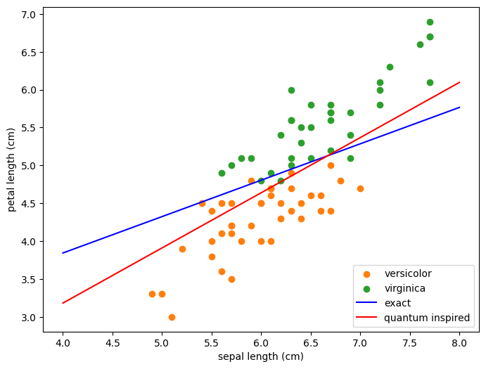
図を描画する#
上記で求めたNumPyによる解\(\theta\)と,量子インスパイアード古典アルゴリズムによる近似解\(\tilde{\theta}\)について, 直線を引いてみて,その様子を見てみます.
[8]:
def line(theta, x):
    return -(theta[0] + theta[1]*x)/theta[2]
[9]:
plt.figure(figsize=(8,6))

# 点を描画する
class1_xs, class1_ys = [], []
class2_xs, class2_ys = [], []
for xt, yt in zip(x_train, y_train):
    if yt == 1:
        class1_xs.append(xt[0])
        class1_ys.append(xt[2])
    else:
        class2_xs.append(xt[0])
        class2_ys.append(xt[2])

plt.scatter(class1_xs, class1_ys, label=iris.target_names[1], color='tab:orange')
plt.scatter(class2_xs, class2_ys, label=iris.target_names[2], color='tab:green')

# 直線を描画する
xs         = np.linspace(4,8)
line_exact = [line(exact_theta, x) for x in xs] # NumPy
line_qi    = [line(tilde_theta, x) for x in xs] # 量子インスパイアード

plt.plot(xs, line_exact, color='blue', label="exact")
plt.plot(xs, line_qi   , color='red',  label="quantum inspired")

# その他
plt.legend(loc='lower right')
plt.xlabel(iris.feature_names[0])
plt.ylabel(iris.feature_names[2])
plt.show()
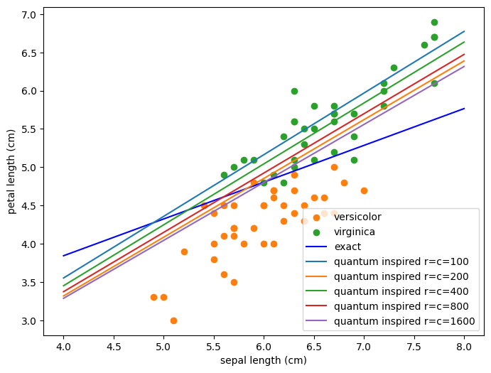
サンプリング回数を増やした時の様子#
[10]:
from quantum_inspired import MatrixBasedDataStructure, SQx
SQA = MatrixBasedDataStructure(A)
sq_theta100  = SQx(SQA, b, 100, 100, 2, 100)
sq_theta200  = SQx(SQA, b, 200, 200, 2, 200)
sq_theta400  = SQx(SQA, b, 400, 400, 2, 400)
sq_theta800  = SQx(SQA, b, 800, 800, 2, 800)
sq_theta1600 = SQx(SQA, b, 1600, 1600, 2, 1600)
[11]:
tilde_theta100  = np.array([sq_theta100.query(i) for i in range(n)])
tilde_theta200  = np.array([sq_theta200.query(i) for i in range(n)])
tilde_theta400  = np.array([sq_theta400.query(i) for i in range(n)])
tilde_theta800  = np.array([sq_theta800.query(i) for i in range(n)])
tilde_theta1600 = np.array([sq_theta1600.query(i) for i in range(n)])
[12]:
plt.figure(figsize=(8,6))

# 点を描画する
class1_xs, class1_ys = [], []
class2_xs, class2_ys = [], []
for xt, yt in zip(x_train, y_train):
    if yt == 1:
        class1_xs.append(xt[0])
        class1_ys.append(xt[2])
    else:
        class2_xs.append(xt[0])
        class2_ys.append(xt[2])

plt.scatter(class1_xs, class1_ys, label=iris.target_names[1], color='tab:orange')
plt.scatter(class2_xs, class2_ys, label=iris.target_names[2], color='tab:green')

# 直線を描画する
xs         = np.linspace(4,8)
line_exact = [line(exact_theta, x) for x in xs]       # NumPy

# 量子インスパイアード
line_qi100 = [line(tilde_theta100, x) for x in xs]
line_qi200 = [line(tilde_theta200, x) for x in xs]
line_qi400 = [line(tilde_theta400, x) for x in xs]
line_qi800 = [line(tilde_theta800, x) for x in xs]
line_qi1600 = [line(tilde_theta1600, x) for x in xs]

plt.plot(xs, line_exact,  color='blue', label="exact")
plt.plot(xs, line_qi100,  label="quantum inspired r=c=100")
plt.plot(xs, line_qi200,  label="quantum inspired r=c=200")
plt.plot(xs, line_qi400,  label="quantum inspired r=c=400")
plt.plot(xs, line_qi800,  label="quantum inspired r=c=800")
plt.plot(xs, line_qi1600, label="quantum inspired r=c=1600")

# その他
plt.legend(loc='lower right')
plt.xlabel(iris.feature_names[0])
plt.ylabel(iris.feature_names[2])
plt.show()
予測#
新しいデータ\((x, y)\)が来たときに,どちらのクラス(versicolor(1)かvirginica(2))に属するかどうかは,\(f(x,y) = \theta_0 + \theta_1 x + \theta_2 y = (\theta_0,\theta_1,\theta_2)^\top (1, x, y)\)の正負によって決定します.
[13]:
from sklearn.metrics import accuracy_score

def f(theta, x, y):
    fx = np.vdot(theta, np.array([1, x, y]))
    if fx > 0:
        return 1
    else:
        return 2
テスト用データに対する予測値を計算します.
[14]:
prediction = []
for xt in x_test:
    c = f(exact_theta, xt[0], xt[2])
    prediction.append(c)
prediction
[14]:
[2, 2, 2, 2, 2, 1, 1, 2, 2, 2, 2, 1, 2, 2, 2, 1, 1, 1, 2, 1, 1, 1, 2, 2, 1]
上記のpredictionがy_testと同様であるか確認してみます.
[15]:
y_test
[15]:
array([2, 2, 1, 2, 2, 1, 1, 2, 2, 2, 2, 1, 2, 2, 2, 1, 1, 1, 2, 1, 1, 2,
       2, 2, 1])
正解率を計算してみます.
[16]:
accuracy_score(y_test, prediction)
[16]:
0.92
次に量子インスパイアード古典アルゴリズムについて考察します. 内積をそのまま計算すると,行列のサイズ分だけ計算量を必要とします. そこで,内積の推定を用いて,\(f(x,y)\)の値を推定し,その推定値に基づいて,どちらのクラスであるか識別します:
[18]:
def qi_vdot(SQa, Qb, sample_size=100):
    val = 0
    for _ in range(sample_size):
        i  = SQa.sample()
        zi = Qb[i]/SQa.query(i)
        val += zi
    return val/sample_size * SQa.norm()**2

def qi_f(SQtheta, x, y, sample_size=100):
    fx = qi_vdot(SQtheta, np.array([1, x, y]), sample_size)
    if fx > 0:
        return 1
    else:
        return 2

xt = x_test[0]
v = np.array([1, xt[0], xt[2]])
qi_vdot(sq_theta, v, 100)
[18]:
0.0
テスト用データに対する予測値を計算します.
[19]:
sq_theta = SQx(SQA, b, 100, 100, 2, 100)

prediction_qi = []
for xt in x_test:
    c = qi_f(sq_theta, xt[0], xt[2], 10)
    prediction_qi.append(c)
prediction_qi
[19]:
[2, 2, 2, 2, 1, 2, 2, 2, 1, 2, 2, 1, 2, 2, 2, 2, 2, 2, 2, 2, 2, 2, 2, 2, 2]
正解率を計算してみます.
[20]:
accuracy_score(y_test, prediction_qi)
[20]:
0.56
参考文献#
András Gilyén, Seth Lloyd, and Ewin Tang, ‘’Quantum-inspired low-rank stochastic regression with logarithmic dependence on the dimension,’’ arXiv:1811.04909, (2018). https://arxiv.org/abs/1811.04909
Ewin Tang. 2019. A quantum-inspired classical algorithm for recommendation systems. In Proceedings of the 51st Annual ACM SIGACT Symposium on Theory of Computing (STOC 2019). Association for Computing Machinery, New York, NY, USA, 217–228. https://doi.org/10.1145/3313276.3316310
平井有三, 「はじめてのパターン認識」, 森北出版, (2012)
[ ]: