量子ソフトウェア勉強会:「量子インスパイアード古典アルゴリズム」ハンズオン資料 1
2023年9月20日(水)
高比良宗一 (名城大学情報工学部情報工学科)

\(\mathrm{SQ}(A)\)と\(\mathrm{SQ}(b)\)の実装について#

このノートブックでは，SQデータ構造を実装します．最初にセグメント木構造を実装します．次に，それを用いてベクトルに基づくデータ構造\(\mathrm{SQ}(v)\)を実装します．その後に行列に基づくデータ構造\(\mathrm{SQ}(A)\)を，ベクトルに基づくデータ構造を用いて実装します．

\[% ![image.png](attachment:image.png) \newcommand{\abs}[1]{|#1|} \newcommand{\norm}[1]{\lVert#1\rVert}\]

[125]:

import random
import math
import numpy as np
import matplotlib.pyplot as plt

セグメント木構造の実装#

セグメント木構造は，次のセルのように実装できます．

[126]:

class SegmentTree:
    def __init__(self, n):
        self.size   = 2**(math.ceil(math.log2(n)) + 1)
        self.height = math.ceil(math.log2(n))
        self.data   = np.zeros(self.size)

    def root(self):
        return self.data[1]

    def leaf(self, i):
        index = self.size//2 + i
        return self.data[index]

    def update(self, k, val):
        size = self.size
        for _ in (range(self.height+1)):
            size = size//2
            self.data[size + k] += val
            k = k // 2

    def __str__(self):
        return str(self.data)

ベクトルに関するデータ構造 \(\mathrm{SQ}(v)\) の実装#

セグメント木構造を用いて，ベクトルに基づいたデータ構造\(\mathrm{SQ}(v)\)を実装します．簡単のために実ベクトルのみを扱います．

定義#

\(\mathrm{SQ}(v)\)の定義は下記の通りです．

ベクトル\(v \in \mathbb{C}^n\)に対して，\(\mathrm{SQ}(v)\)を次の操作(1-3)が行えるようなデータ構造とする．(2.のDefinition 2.5や3.のDefinition 1.1など) - \(\text{Sample}()\). 確率\(\abs{v_i}^2/\norm{v}^2\)で添字\(i\)を出力する - \(\text{Query}(i)\). ベクトルの第\(i\)成分を出力する - \(\text{Norm}()\). ベクトルの2ノルム\(\norm{v}\)を出力する

実装#

[127]:

class VectorBasedDataStructure:
    def __init__(self, vector):
        self.n = vector.size
        self.segment_tree = SegmentTree(self.n)
        self.sgn = np.sign(vector)
        for i in range(self.n):
            self.segment_tree.update(i, abs(vector[i])**2)

    def sample(self):
        return self._sample2()

    def _sample1(self):
        height = self.segment_tree.height
        size   = self.segment_tree.size
        k = 1
        for _ in range(height):
            if random.random() < self.segment_tree.data[2*k]/self.segment_tree.data[k]:
                k = 2*k
            else:
                k = 2*k+1
        return k - size//2

    def _sample2(self):
        height = self.segment_tree.height
        size   = self.segment_tree.size
        k = 1
        for _ in range(height):
            if random.random()*self.segment_tree.data[k] < self.segment_tree.data[2*k]:
                k = 2*k
            else:
                k = 2*k+1
        return k - size//2

    def query(self, i):
        val = self.segment_tree.leaf(i)
        return self.sgn[i]*math.sqrt(val)

    def norm(self):
        return math.sqrt(self.segment_tree.root())

    def print_structure(self):
        data = self.segment_tree.data
        height = self.segment_tree.height
        print("height =", height)
        k = 1
        for i in range(height+1):
            lst = []
            for j in range(2**i,2**(i+1)):
                lst.append(data[j])
            print(lst)
        print(self.sgn)

確認#

上のセルのVectorBasedDataStructureが\(\mathrm{SQ}(v)\)を実装できているか確認します．各関数\(\mathrm{Norm}(), \mathrm{Query}(i), \mathrm{Sample}()\)それぞれについて確認していきます．

[128]:

import numpy as np
n = 10
v = np.random.rand(n) - np.random.rand(n)
SQv = VectorBasedDataStructure(v)

[129]:

SQv.print_structure()

height = 4
[2.448569350113205]
[1.8257522517986355, 0.6228170983145696]
[1.4081692953908433, 0.417582956407792, 0.6228170983145696, 0.0]
[0.9040148948790538, 0.5041544005117894, 0.18858400987600943, 0.2289989465317826, 0.6228170983145696, 0.0, 0.0, 0.0]
[0.5134774824972979, 0.390537412381756, 0.5012377704182622, 0.0029166300935271807, 0.1416840701326077, 0.046899939743401745, 0.2107787982003918, 0.018220148331390806, 0.4618647517187302, 0.16095234659583932, 0.0, 0.0, 0.0, 0.0, 0.0, 0.0]
[-1. -1. -1. -1.  1. -1. -1. -1. -1.  1.]

\(\mathrm{Norm}()\)について#

ベクトルの2ノルムが計算できているかどうか，NumPyの結果と比較をして確認してみます．

[130]:

val = SQv.norm()
normv = np.linalg.norm(v, 2)

print(f"SQv.norm() = {val},\nnumpy.linalg.norm(v) = {normv}")

SQv.norm() = 1.5647905131720363,
numpy.linalg.norm(v) = 1.5647905131720363

\(\mathrm{Query}(i)\)について#

全ての\(i\)に対して，元々のベクトル\(v\)の\(i\)番目の成分と比較をしてみます．

[131]:

for i in range(n):
    val = SQv.query(i)
    vi  = v[i]
    print(f"SQv.query({i}) = {val}, v_{i} = {vi}")

test_vector = np.array([SQv.query(i) for i in range(n)])
np.allclose(test_vector, v)

SQv.query(0) = -0.7165734313364527, v_0 = -0.7165734313364527
SQv.query(1) = -0.6249299259771098, v_1 = -0.6249299259771098
SQv.query(2) = -0.7079814760417551, v_2 = -0.7079814760417551
SQv.query(3) = -0.05400583388419422, v_3 = -0.05400583388419422
SQv.query(4) = 0.37640944479729477, v_4 = 0.37640944479729477
SQv.query(5) = -0.21656393915747318, v_5 = -0.21656393915747318
SQv.query(6) = -0.4591065216269442, v_6 = -0.4591065216269442
SQv.query(7) = -0.13498202966095452, v_7 = -0.13498202966095452
SQv.query(8) = -0.6796063211291742, v_8 = -0.6796063211291742
SQv.query(9) = 0.4011886670830064, v_9 = 0.4011886670830064

[131]:

True

\(\mathrm{Sample}()\)について#

SQv.sample()を何度も実行して得られた結果と，真の確率分布\(\mathcal{D}_v (\Pr(i) = |v_i|^2/\norm{v}^2)\)とを比較します．

[132]:

normv = np.linalg.norm(v, 2)
Dv = np.array([abs(v[i])**2/normv**2 for i in range(n)])

counts = np.zeros(n)

sample_size = 10000
for _ in range(sample_size):
    i = SQv.sample()
    counts[i] += 1

print("SQ(v)", counts/sample_size)
print("exact", Dv)

print("error =", np.linalg.norm(Dv - counts/sample_size))

plt.figure(figsize=(8,6))
plt.bar(range(n), counts/sample_size, alpha=0.7, label="SQ(v).sample()")
plt.bar(range(n), Dv                , alpha=0.6, label="Dv(exact)")

plt.legend()
plt.xlabel("index i")
plt.show()

SQ(v) [0.2141 0.162  0.2029 0.0014 0.0574 0.0196 0.089  0.008  0.183  0.0626]
exact [0.2097051  0.15949616 0.20470638 0.00119116 0.05786402 0.01915402
 0.08608243 0.00744114 0.18862637 0.06573322]
error = 0.008922043102418013

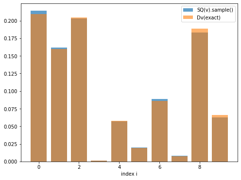
../_images/notebooks_08_01_Data_structure_15_1.png

グラフの青色は\(\mathrm{SQ}(v)\)の結果を表し，オレンジ色は真の分布\(\mathcal{D}_v\)を表します．視覚的に見て大体同じであることを確認できると思います．

行列に基づくデータ構造 \(\mathrm{SQ}(A)\) の実装#

\(\mathrm{SQ}(v)\)について実装しました．これを用いて\(\mathrm{SQ}(A)\)を実装します．簡単のために実行列のみを扱います．

定義#

行列\(A \in \mathbb{C}^{m \times n}\)に対して，\(\mathrm{SQ}(A)\)を次の操作(1-5)が行えるようなデータ構造とする．(2.のDefinition 2.10や3.のDefinition 1.2など) - \(\text{Sample1}()\). 確率\(\norm{A_{i,\ast}}^2/\norm{A}_\mathrm{F}^2\)で行添字\(i\)を出力する - \(\text{Sample2}(i)\). 確率\(\abs{A_{ij}}^2/\norm{A_{i,\ast}}^2\)で列添字\(j\)を出力する - \(\text{Query}(i,j)\). 第\((i,j)\)成分\(A_{ij}\)を出力する - \(\text{Norm}(i)\). 第\(i\)行の2ノルム\(\norm{A_{i,\ast}}\)を出力する - \(\text{Norm}()\). フロべニウスノルム\(\norm{A}_\mathrm{F}\)を出力する

実装#

VectorBasedDataStructureを用いて\(\mathrm{SQ(A)}\)を実装します．

[133]:

class MatrixBasedDataStructure:
    def __init__(self, matrix):
        self.m, self.n = matrix.shape
        self.shape = matrix.shape

        self.vecFro = np.array([np.linalg.norm(matrix[i,:]) for i in range(self.m)])
        self.SQvecFro = VectorBasedDataStructure(self.vecFro)
        self.SQrowlist = [VectorBasedDataStructure(matrix[i,:]) for i in range(self.m)]


    def sample1(self):
        return self.SQvecFro.sample()

    def sample2(self, i):
        return self.SQrowlist[i].sample()

    def query(self, i, j):
        return self.SQrowlist[i].query(j)

    def norm(self, i):
        return self.SQrowlist[i].norm()

    def normF(self):
        return self.SQvecFro.norm()

確認#

上のセルのMatrixBasedDataStructureが\(\mathrm{SQ}(A)\)を実装できているか確認します．各関数\(\mathrm{Sample1}()\), \(\mathrm{Sample2}()\), \(\mathrm{Query}()\), \(\mathrm{Norm}(i)\), \(\mathrm{Norm}()\) (normF), それぞれ確認していきます．

[134]:

m, n = 8, 16
A = np.random.rand(m, n) - np.random.rand(m, n)
SQA = MatrixBasedDataStructure(A)

\(\mathrm{Sample1}()\)について#

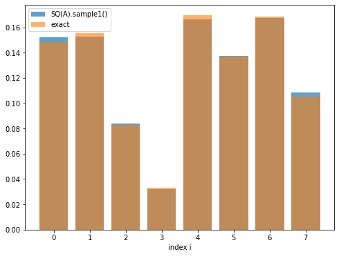
SQA.sample1()を何度も実行して得られた結果と，真の確率分布\(\Pr(i) = \norm{A_{i,\ast}}^2/\norm{A}_\mathrm{F}^2\)とを比較します．

[135]:

normAF = np.linalg.norm(A) # Aのフロべニウスノルム
Da = np.array([np.linalg.norm(A[i,:])**2/normAF**2 for i in range(m)])

sample_size = 10000
counts = np.zeros(m)
for _ in range(sample_size):
    i = SQA.sample1()
    counts[i] += 1

print("SQ(A).sample1()\n", counts/sample_size)
print("exact\n", Da)
print("error =", np.linalg.norm(Da - counts/sample_size))

plt.figure(figsize=(8,6))

plt.bar(range(m), counts/sample_size, alpha=0.7, label="SQ(A).sample1()")
plt.bar(range(m), Da,                 alpha=0.6, label="exact")

plt.legend()
plt.xlabel("index i")
plt.show()

SQ(A).sample1()
 [0.1522 0.1526 0.0841 0.032  0.1664 0.1372 0.1672 0.1083]
exact
 [0.14825435 0.15554245 0.08303897 0.03323757 0.16950496 0.1370892
 0.16827819 0.10505432]
error = 0.006945032299413305

../_images/notebooks_08_01_Data_structure_24_1.png

\(\mathrm{Sample2}(i)\)について#

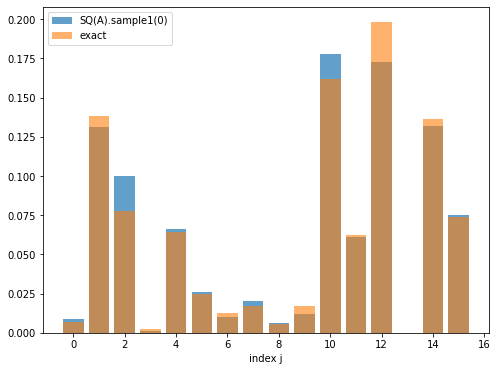
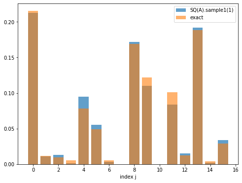
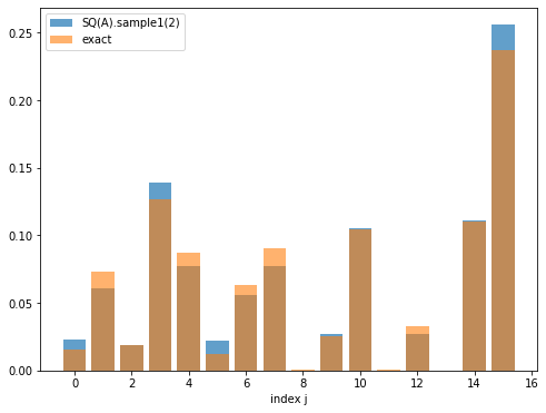
\(\mathrm{Sample2}(i)\)について確認します．\(i = 0,1,2,\dots,m-1\)の全てを調査すると図がたくさん表示されるので，図については\(i=0,1,2\)までを見ます． SQA.sample2()を何度も実行して得られた結果と，真の確率分布\(\Pr(j) = |A_{i,j}|^2/\norm{A_{i,\ast}}^2)\)とを比較します．

[136]:

sample_size = 1000
for i in range(m):
    normAi = np.linalg.norm(A[i,:])
    Dai = np.array([abs(A[i,j])**2/normAi**2 for j in range(n)])

    counts = np.zeros(n)
    for _ in range(sample_size):
        j = SQA.sample2(i)
        counts[j] += 1

    print(f"--------- i = {i} ----------")
    print(f"SQ(A).sample2({i}):\n", counts/sample_size)
    print("exact:\n", Dai)
    print("error =", np.linalg.norm(Dai - counts/sample_size))

    if i < 3:
        plt.figure(figsize=(8,6))
        plt.bar(range(n), counts/sample_size, alpha=0.7, label=f"SQ(A).sample1({i})")
        plt.bar(range(n), Dai, alpha=0.6, label="exact")
        plt.legend()
        plt.xlabel("index j")
        plt.show()

--------- i = 0 ----------
SQ(A).sample2(0):
 [0.009 0.131 0.1   0.001 0.066 0.026 0.01  0.02  0.006 0.012 0.178 0.061
 0.173 0.    0.132 0.075]
exact:
 [6.67122278e-03 1.38546480e-01 7.76453219e-02 2.50954261e-03
 6.44932654e-02 2.45554475e-02 1.28339181e-02 1.72999979e-02
 5.34582623e-03 1.68245798e-02 1.62068438e-01 6.26758781e-02
 1.98143792e-01 6.71504133e-07 1.36248853e-01 7.41367652e-02]
error = 0.038928099973546876

../_images/notebooks_08_01_Data_structure_26_1.png

--------- i = 1 ----------
SQ(A).sample2(1):
 [0.213 0.011 0.013 0.001 0.095 0.055 0.003 0.    0.172 0.11  0.    0.084
 0.015 0.192 0.002 0.034]
exact:
 [2.15359578e-01 1.16837036e-02 9.31491496e-03 5.06239791e-03
 7.80504864e-02 4.90597131e-02 5.19151565e-03 2.48252261e-06
 1.69286768e-01 1.21914890e-01 4.32025218e-05 1.00895384e-01
 1.23973871e-02 1.88623411e-01 3.99739544e-03 2.91167693e-02]
error = 0.029056605818409322

../_images/notebooks_08_01_Data_structure_26_3.png

--------- i = 2 ----------
SQ(A).sample2(2):
 [0.023 0.061 0.019 0.139 0.077 0.022 0.056 0.077 0.    0.027 0.105 0.
 0.027 0.    0.111 0.256]
exact:
 [1.57269980e-02 7.35258294e-02 1.89341155e-02 1.26425068e-01
 8.75346716e-02 1.25606000e-02 6.36604968e-02 9.08985281e-02
 7.63685414e-04 2.50247356e-02 1.04376861e-01 2.50924759e-04
 3.29819512e-02 2.76470713e-05 1.09891470e-01 2.37416418e-01]
error = 0.034744195213902936

../_images/notebooks_08_01_Data_structure_26_5.png

--------- i = 3 ----------
SQ(A).sample2(3):
 [0.154 0.002 0.018 0.055 0.03  0.019 0.143 0.019 0.18  0.038 0.045 0.008
 0.    0.154 0.135 0.   ]
exact:
 [1.69432833e-01 1.60980102e-03 1.10291568e-02 5.21402355e-02
 3.43614356e-02 1.78829232e-02 1.56175123e-01 1.28661022e-02
 1.77819918e-01 3.81903573e-02 3.70157725e-02 1.25719260e-02
 1.25468382e-04 1.56160672e-01 1.22569680e-01 4.85963581e-05]
error = 0.027842645049913007
--------- i = 4 ----------
SQ(A).sample2(4):
 [0.014 0.017 0.088 0.004 0.003 0.057 0.017 0.058 0.025 0.065 0.001 0.176
 0.214 0.055 0.037 0.169]
exact:
 [0.01393605 0.0217129  0.07857658 0.00524667 0.0040309  0.05020077
 0.02124284 0.05733651 0.02595176 0.07900304 0.00195552 0.17700639
 0.21686669 0.05330799 0.04394615 0.14967925]
error = 0.02845773519419411
--------- i = 5 ----------
SQ(A).sample2(5):
 [0.013 0.047 0.012 0.    0.017 0.014 0.102 0.11  0.001 0.03  0.033 0.15
 0.097 0.011 0.082 0.281]
exact:
 [0.01576997 0.04215698 0.01144164 0.00033565 0.01556054 0.01639636
 0.10100832 0.10008773 0.0014015  0.02666267 0.03470309 0.1538619
 0.10978272 0.00868706 0.07262467 0.2895192 ]
error = 0.022292108031832302
--------- i = 6 ----------
SQ(A).sample2(6):
 [0.005 0.034 0.252 0.027 0.03  0.001 0.041 0.027 0.153 0.021 0.132 0.
 0.004 0.022 0.153 0.098]
exact:
 [0.0052013  0.03883059 0.27740928 0.02884997 0.02194162 0.00064374
 0.03472452 0.02751076 0.1596721  0.02511733 0.11893572 0.00081955
 0.00126794 0.01839077 0.13991555 0.10076927]
error = 0.034775200605602186
--------- i = 7 ----------
SQ(A).sample2(7):
 [0.003 0.137 0.065 0.24  0.    0.052 0.073 0.008 0.045 0.016 0.03  0.044
 0.219 0.003 0.001 0.064]
exact:
 [0.00434803 0.13924038 0.08037212 0.23336496 0.00033546 0.04986425
 0.05077556 0.00809676 0.05716576 0.01563804 0.03255437 0.04650511
 0.21055747 0.00359115 0.00176015 0.06583043]
error = 0.03197284358965613

\(\mathrm{Query}(i,j)\)について#

全ての\(i,j\)に対して，元々の行列\(A\)の\(i,j\)番目の成分と比較をしていきます．

[137]:

for i in range(m):
    for j in range(n):
        val = SQA.query(i,j)
        Aij = A[i, j]
        print(f"SQA.query({i},{j}) = {val}, A[{i},{j}] = {Aij}")

test_matrix = np.array([[SQA.query(i,j) for j in range(n)] for i in range(m)])
np.allclose(test_matrix, A)

SQA.query(0,0) = 0.14093412328130706, A[0,0] = 0.14093412328130706
SQA.query(0,1) = -0.6422604567828589, A[0,1] = -0.6422604567828589
SQA.query(0,2) = 0.4808073338826254, A[0,2] = 0.4808073338826254
SQA.query(0,3) = 0.08643919692093416, A[0,3] = 0.08643919692093416
SQA.query(0,4) = 0.438198230360778, A[0,4] = 0.438198230360778
SQA.query(0,5) = 0.2703879684103896, A[0,5] = 0.2703879684103896
SQA.query(0,6) = 0.1954758311642607, A[0,6] = 0.1954758311642607
SQA.query(0,7) = 0.22695327908324625, A[0,7] = 0.22695327908324625
SQA.query(0,8) = 0.12615976025407138, A[0,8] = 0.12615976025407138
SQA.query(0,9) = -0.2238131242581275, A[0,9] = -0.2238131242581275
SQA.query(0,10) = 0.694644592086265, A[0,10] = 0.694644592086265
SQA.query(0,11) = 0.4319800096257096, A[0,11] = 0.4319800096257096
SQA.query(0,12) = -0.7680750739709041, A[0,12] = -0.7680750739709041
SQA.query(0,13) = 0.0014139621405123703, A[0,13] = 0.0014139621405123703
SQA.query(0,14) = 0.6369126347355241, A[0,14] = 0.6369126347355241
SQA.query(0,15) = 0.46981864981002985, A[0,15] = 0.46981864981002985
SQA.query(1,0) = -0.8201933963741046, A[1,0] = -0.8201933963741046
SQA.query(1,1) = 0.19104005693382153, A[1,1] = 0.19104005693382153
SQA.query(1,2) = 0.17057823648830006, A[1,2] = 0.17057823648830006
SQA.query(1,3) = 0.12575125033809176, A[1,3] = 0.12575125033809176
SQA.query(1,4) = -0.49376690737214046, A[1,4] = -0.49376690737214046
SQA.query(1,5) = -0.39146836758388903, A[1,5] = -0.39146836758388903
SQA.query(1,6) = 0.12734481200033876, A[1,6] = 0.12734481200033876
SQA.query(1,7) = 0.0027847151601838593, A[1,7] = 0.0027847151601838593
SQA.query(1,8) = -0.7271862858557843, A[1,8] = -0.7271862858557843
SQA.query(1,9) = -0.6171099494546467, A[1,9] = -0.6171099494546467
SQA.query(1,10) = -0.011616859101067578, A[1,10] = -0.011616859101067578
SQA.query(1,11) = -0.5613966577861469, A[1,11] = -0.5613966577861469
SQA.query(1,12) = 0.19678829123864472, A[1,12] = 0.19678829123864472
SQA.query(1,13) = -0.7675947054442894, A[1,13] = -0.7675947054442894
SQA.query(1,14) = 0.1117436181422381, A[1,14] = 0.1117436181422381
SQA.query(1,15) = 0.30158224234842623, A[1,15] = 0.30158224234842623
SQA.query(2,0) = 0.16194726362509615, A[2,0] = 0.16194726362509615
SQA.query(2,1) = -0.3501633308703348, A[2,1] = -0.3501633308703348
SQA.query(2,2) = -0.17769418248106894, A[2,2] = -0.17769418248106894
SQA.query(2,3) = 0.4591634344249518, A[2,3] = 0.4591634344249518
SQA.query(2,4) = -0.3820680765301999, A[2,4] = -0.3820680765301999
SQA.query(2,5) = 0.14472911011702605, A[2,5] = 0.14472911011702605
SQA.query(2,6) = -0.325825980138746, A[2,6] = -0.325825980138746
SQA.query(2,7) = 0.3893400890919879, A[2,7] = 0.3893400890919879
SQA.query(2,8) = 0.03568682789941191, A[2,8] = 0.03568682789941191
SQA.query(2,9) = 0.2042845148393685, A[2,9] = 0.2042845148393685
SQA.query(2,10) = 0.41720817959265766, A[2,10] = 0.41720817959265766
SQA.query(2,11) = 0.020456082024582822, A[2,11] = 0.020456082024582822
SQA.query(2,12) = 0.2345248521009452, A[2,12] = 0.2345248521009452
SQA.query(2,13) = -0.006790085839027404, A[2,13] = -0.006790085839027404
SQA.query(2,14) = -0.4280876401967807, A[2,14] = -0.4280876401967807
SQA.query(2,15) = -0.6292251501525093, A[2,15] = -0.6292251501525093
SQA.query(3,0) = 0.3362970843015157, A[3,0] = 0.3362970843015157
SQA.query(3,1) = -0.032780110699528464, A[3,1] = -0.032780110699528464
SQA.query(3,2) = 0.08580161676563114, A[3,2] = 0.08580161676563114
SQA.query(3,3) = -0.18655668248293644, A[3,3] = -0.18655668248293644
SQA.query(3,4) = -0.15144675283966347, A[3,4] = -0.15144675283966347
SQA.query(3,5) = -0.10925556615764154, A[3,5] = -0.10925556615764154
SQA.query(3,6) = 0.3228718958953265, A[3,6] = 0.3228718958953265
SQA.query(3,7) = -0.09267184619828961, A[3,7] = -0.09267184619828961
SQA.query(3,8) = 0.34452006368823207, A[3,8] = 0.34452006368823207
SQA.query(3,9) = 0.15966185725909277, A[3,9] = 0.15966185725909277
SQA.query(3,10) = 0.15718739802730652, A[3,10] = 0.15718739802730652
SQA.query(3,11) = -0.09160627519329856, A[3,11] = -0.09160627519329856
SQA.query(3,12) = 0.009151482736465266, A[3,12] = 0.009151482736465266
SQA.query(3,13) = 0.32285695830253747, A[3,13] = 0.32285695830253747
SQA.query(3,14) = 0.2860328029573471, A[3,14] = 0.2860328029573471
SQA.query(3,15) = 0.0056954255366680195, A[3,15] = 0.0056954255366680195
SQA.query(4,0) = 0.21780649015659348, A[4,0] = 0.21780649015659348
SQA.query(4,1) = 0.2718690747371104, A[4,1] = 0.2718690747371104
SQA.query(4,2) = 0.5171868597757535, A[4,2] = 0.5171868597757535
SQA.query(4,3) = -0.13364197820892265, A[4,3] = -0.13364197820892265
SQA.query(4,4) = -0.11713908379811988, A[4,4] = -0.11713908379811988
SQA.query(4,5) = 0.4133863403370368, A[4,5] = 0.4133863403370368
SQA.query(4,6) = 0.2689101696622659, A[4,6] = 0.2689101696622659
SQA.query(4,7) = 0.4417906533895565, A[4,7] = 0.4417906533895565
SQA.query(4,8) = -0.2972243018824269, A[4,8] = -0.2972243018824269
SQA.query(4,9) = 0.518588424140816, A[4,9] = 0.518588424140816
SQA.query(4,10) = -0.0815890485970916, A[4,10] = -0.0815890485970916
SQA.query(4,11) = -0.776238874583782, A[4,11] = -0.776238874583782
SQA.query(4,12) = -0.8592060710086514, A[4,12] = -0.8592060710086514
SQA.query(4,13) = 0.4259876904483514, A[4,13] = 0.4259876904483514
SQA.query(4,14) = -0.38677759652068755, A[4,14] = -0.38677759652068755
SQA.query(4,15) = 0.7138084930173041, A[4,15] = 0.7138084930173041
SQA.query(5,0) = 0.20836592388937025, A[5,0] = 0.20836592388937025
SQA.query(5,1) = 0.34067956078481576, A[5,1] = 0.34067956078481576
SQA.query(5,2) = 0.17748247527291805, A[5,2] = 0.17748247527291805
SQA.query(5,3) = 0.030398627777401765, A[5,3] = 0.030398627777401765
SQA.query(5,4) = -0.20697775838029697, A[5,4] = -0.20697775838029697
SQA.query(5,5) = 0.21246383998474372, A[5,5] = 0.21246383998474372
SQA.query(5,6) = -0.5273390168337392, A[5,6] = -0.5273390168337392
SQA.query(5,7) = -0.5249304229808457, A[5,7] = -0.5249304229808457
SQA.query(5,8) = 0.06211661058983631, A[5,8] = 0.06211661058983631
SQA.query(5,9) = 0.27093375338051207, A[5,9] = 0.27093375338051207
SQA.query(5,10) = 0.3090974536216523, A[5,10] = 0.3090974536216523
SQA.query(5,11) = 0.6508439478107384, A[5,11] = 0.6508439478107384
SQA.query(5,12) = 0.549766563407166, A[5,12] = 0.549766563407166
SQA.query(5,13) = -0.15464923556456833, A[5,13] = -0.15464923556456833
SQA.query(5,14) = -0.4471501765864284, A[5,14] = -0.4471501765864284
SQA.query(5,15) = -0.8927914167341512, A[5,15] = -0.8927914167341512
SQA.query(6,0) = -0.13258052903277384, A[6,0] = -0.13258052903277384
SQA.query(6,1) = 0.3622518401646888, A[6,1] = 0.3622518401646888
SQA.query(6,2) = 0.9682424470459597, A[6,2] = 0.9682424470459597
SQA.query(6,3) = 0.3122455850735979, A[6,3] = 0.3122455850735979
SQA.query(6,4) = -0.27230647328439617, A[6,4] = -0.27230647328439617
SQA.query(6,5) = -0.04664235819021334, A[6,5] = -0.04664235819021334
SQA.query(6,6) = 0.34256403322217643, A[6,6] = 0.34256403322217643
SQA.query(6,7) = -0.3049122587462949, A[6,7] = -0.3049122587462949
SQA.query(6,8) = 0.7345783762682324, A[6,8] = 0.7345783762682324
SQA.query(6,9) = -0.29134688974415235, A[6,9] = -0.29134688974415235
SQA.query(6,10) = 0.6339861653430977, A[6,10] = 0.6339861653430977
SQA.query(6,11) = -0.05262732554989691, A[6,11] = -0.05262732554989691
SQA.query(6,12) = -0.06545946168630756, A[6,12] = -0.06545946168630756
SQA.query(6,13) = 0.2493007349621853, A[6,13] = 0.2493007349621853
SQA.query(6,14) = -0.6876328511517561, A[6,14] = -0.6876328511517561
SQA.query(6,15) = -0.5835629175555761, A[6,15] = -0.5835629175555761
SQA.query(7,0) = -0.0957773323822696, A[7,0] = -0.0957773323822696
SQA.query(7,1) = 0.5419999670745368, A[7,1] = 0.5419999670745368
SQA.query(7,2) = 0.41178392385220786, A[7,2] = 0.41178392385220786
SQA.query(7,3) = 0.7016725469592794, A[7,3] = 0.7016725469592794
SQA.query(7,4) = -0.02660351905816538, A[7,4] = -0.02660351905816538
SQA.query(7,5) = -0.324348058898821, A[7,5] = -0.324348058898821
SQA.query(7,6) = -0.3272985056145026, A[7,6] = -0.3272985056145026
SQA.query(7,7) = 0.13069902444473547, A[7,7] = 0.13069902444473547
SQA.query(7,8) = 0.34728390209753224, A[7,8] = 0.34728390209753224
SQA.query(7,9) = -0.18163848348933354, A[7,9] = -0.18163848348933354
SQA.query(7,10) = 0.26207242647626483, A[7,10] = 0.26207242647626483
SQA.query(7,11) = 0.31323262604248814, A[7,11] = 0.31323262604248814
SQA.query(7,12) = -0.6665028152726765, A[7,12] = -0.6665028152726765
SQA.query(7,13) = 0.08704291439877654, A[7,13] = 0.08704291439877654
SQA.query(7,14) = -0.0609384398900068, A[7,14] = -0.0609384398900068
SQA.query(7,15) = -0.3726747743755001, A[7,15] = -0.3726747743755001

[137]:

True

\(\mathrm{Norm}(i)\)について#

行列\(A\)の各列ベクトル\(A_{0,\ast},\dots,A_{m,\ast}\)の2ノルムが計算できているかどうか，NumPyの関数を用いた時の結果と比較をして確認してみます．

[138]:

for i in range(m):
    val    = SQA.norm(i)
    normAi =  np.linalg.norm(A[i,:])
    print(f"SQ(A).norm({i}) = {val} \t, np.linalg.norm(Ai) = {normAi}")

SQ(A).norm(0) = 1.7254939312579298      , np.linalg.norm(Ai) = 1.7254939312579296
SQ(A).norm(1) = 1.7673972420715773      , np.linalg.norm(Ai) = 1.7673972420715773
SQ(A).norm(2) = 1.2913700163394468      , np.linalg.norm(Ai) = 1.2913700163394468
SQ(A).norm(3) = 0.8170042507879813      , np.linalg.norm(Ai) = 0.8170042507879812
SQ(A).norm(4) = 1.84501930629778        , np.linalg.norm(Ai) = 1.8450193062977802
SQ(A).norm(5) = 1.659248081864714       , np.linalg.norm(Ai) = 1.6592480818647137
SQ(A).norm(6) = 1.8383306476239845      , np.linalg.norm(Ai) = 1.8383306476239842
SQ(A).norm(7) = 1.452501744169358       , np.linalg.norm(Ai) = 1.452501744169358

\(\mathrm{Norm}()\)について#

行列のフロべニウスノルムが計算できているかどうか，NumPyの関数を用いた時の結果と比較をして確認してみます．

[139]:

print("SQ(A) norm()  ", SQA.normF())
print("Frobenius norm", np.linalg.norm(A))

SQ(A) norm()   4.481358734534456
Frobenius norm 4.481358734534455

まとめ#

\(\mathrm{SQ}(v), \mathrm{SQ}(A)\)をそれぞれVectorBasedDataStructure, MatrixBasedDataStructureで実装しました．

参考文献#

Ewin Tang. 2019. A quantum-inspired classical algorithm for recommendation systems. In Proceedings of the 51st Annual ACM SIGACT Symposium on Theory of Computing (STOC 2019). Association for Computing Machinery, New York, NY, USA, 217–228. https://doi.org/10.1145/3313276.3316310
Nai-Hui Chia, András Gilyén, Tongyang Li, Han-Hsuan Lin, Ewin Tang, and Chunhao Wang. 2020. Sampling-based sublinear low-rank matrix arithmetic framework for dequantizing Quantum machine learning. In Proceedings of the 52nd Annual ACM SIGACT Symposium on Theory of Computing (STOC 2020). Association for Computing Machinery, New York, NY, USA, 387–400. https://doi.org/10.1145/3357713.3384314
András Gilyén, Zhao Song and Ewin Tang. 2022. An improved quantum-inspired algorithm for linear regression. Quantum, 6, 754. https://doi.org/10.22331/q-2022-06-30-754
https://en.wikipedia.org/wiki/Segment_tree

\mathrm{SQ}(A)と\mathrm{SQ}(b)の実装について

Contents

\(\mathrm{SQ}(A)\)と\(\mathrm{SQ}(b)\)の実装について#

セグメント木構造の実装#

ベクトルに関するデータ構造 \(\mathrm{SQ}(v)\) の実装#

定義#

実装#

確認#

\(\mathrm{Norm}()\)について#

\(\mathrm{Query}(i)\)について#

\(\mathrm{Sample}()\)について#

行列に基づくデータ構造 \(\mathrm{SQ}(A)\) の実装#

定義#

実装#

確認#

\(\mathrm{Sample1}()\)について#

\(\mathrm{Sample2}(i)\)について#

\(\mathrm{Query}(i,j)\)について#

\(\mathrm{Norm}(i)\)について#

\(\mathrm{Norm}()\)について#

まとめ#

参考文献#