
\[\newcommand{\norm}[1]{\lVert#1\rVert} \renewcommand{\top}{\mathsf{T}} \newcommand{\SQ}{\mathrm{SQ}}\]# \(x = A^+b\)に関する量子インスパイアード古典アルゴリズム Part 1 ### (行列\(C\)の特異値分解まで)
このノートブックでは,量子インスパイアード古典アルゴリズムにおける,\(A\)から構成される行列\(C\)を得るまでの部分,及びその特異値分解について実装します.そして\(C\)の左特異ベクトル\(w^{(\ell)}\)と特異値\(\tilde{\sigma}\)によって,\(A\)の左右の特異ベクトルと特異値が近似される様子を確認してみます.
行列\(A\)を定義する#
低ランク行列\(A\)を生成する関数を定義します.
[2]:
import random
import cmath, math
import time
import numpy as np
import scipy as sp
import scipy.linalg
import matplotlib.pyplot as plt

def low_rank_matrix(m, n, rank, cond=10):

    """
    ランクが`rank`で,条件数が`cond`であるような m x n の実行列を生成する.
    ここで条件数とは最大特異値/最小特異値である.したがってrank=1のときは条件数の値は1になる.

    """

    U, _  = np.linalg.qr(np.random.rand(m, m))
    Vh, _ = np.linalg.qr(np.random.rand(n, n))

    if rank==1:
        diag = np.array([cond])

    elif rank==2:
        diag = np.array([1, 1/cond])
    else:
        diag = [random.uniform(1/cond, 1) for i in range(rank)]
        diag[1] = 1
        diag[2] = 1/cond

    return U[:,:rank] @ np.diag(diag) @ Vh[:rank,:]
[33]:
m, n = 400, 300
A = low_rank_matrix(m, n, 2, 8)

rankA = np.linalg.matrix_rank(A)
normF = np.linalg.norm(A)
norm2 = np.linalg.norm(A, 2)
svdvals = sp.linalg.svdvals(A)
condnumber = max(svdvals[:rankA])/min(svdvals[:rankA])

print("Aのランク =", rankA)
print("Aのフロべニウスノルム =", normF)
print("Aの2ノルム =", norm2)
print("Aの特異値\n", svdvals)
print("Aの条件数\n", condnumber)
Aのランク = 2
Aのフロべニウスノルム = 1.0077822185373184
Aの2ノルム = 0.9999999999999997
Aの特異値
 [1.00000000e+00 1.25000000e-01 5.19213071e-16 4.79118019e-16
 4.71713714e-16 4.58222417e-16 4.18376202e-16 3.81834822e-16
 3.54408030e-16 3.47628970e-16 3.21416227e-16 3.06267277e-16
 2.94596201e-16 2.77563960e-16 2.60622934e-16 2.58545313e-16
 2.29930845e-16 2.29601626e-16 2.19035211e-16 2.08345819e-16
 2.02803805e-16 1.74125391e-16 1.59430441e-16 1.47403420e-16
 1.44858870e-16 1.29917459e-16 1.17028191e-16 1.00297735e-16
 9.37942832e-17 8.61352464e-17 8.54481002e-17 8.25804231e-17
 8.02026027e-17 7.59935124e-17 6.71003385e-17 6.55470690e-17
 6.29616202e-17 5.99590794e-17 5.90842981e-17 5.83481073e-17
 5.42559429e-17 5.32616988e-17 5.20634581e-17 4.88518527e-17
 4.77845279e-17 4.71140163e-17 4.53903152e-17 4.34603235e-17
 4.18865006e-17 4.11653036e-17 4.03700291e-17 3.93219745e-17
 3.78008155e-17 3.61795232e-17 3.48760210e-17 3.44060987e-17
 3.21714941e-17 3.18224187e-17 3.15013830e-17 3.09899747e-17
 3.05030105e-17 2.94799811e-17 2.87547844e-17 2.82762851e-17
 2.71794738e-17 2.66188204e-17 2.65593766e-17 2.58955778e-17
 2.57313346e-17 2.50097543e-17 2.48568056e-17 2.42186036e-17
 2.40435255e-17 2.36537034e-17 2.35260358e-17 2.30242899e-17
 2.23809209e-17 2.17939005e-17 2.16015771e-17 2.14806951e-17
 2.08692603e-17 2.05871356e-17 2.04536573e-17 2.03399627e-17
 1.95932932e-17 1.94572013e-17 1.92152275e-17 1.89255407e-17
 1.86323067e-17 1.85739870e-17 1.82830250e-17 1.77793150e-17
 1.77569421e-17 1.76039948e-17 1.69915772e-17 1.67849530e-17
 1.65287465e-17 1.64180495e-17 1.62054369e-17 1.58363436e-17
 1.57454327e-17 1.55593677e-17 1.54212713e-17 1.51981088e-17
 1.49675088e-17 1.46895809e-17 1.44847141e-17 1.43737005e-17
 1.41737181e-17 1.40435267e-17 1.38353451e-17 1.37652725e-17
 1.35983264e-17 1.31958979e-17 1.30107535e-17 1.29555106e-17
 1.28594865e-17 1.25156029e-17 1.24675914e-17 1.21872844e-17
 1.21783613e-17 1.19813660e-17 1.19021017e-17 1.16668045e-17
 1.14976212e-17 1.13525816e-17 1.13306028e-17 1.11254143e-17
 1.11109004e-17 1.07572074e-17 1.07482652e-17 1.06404959e-17
 1.04345157e-17 1.02335277e-17 1.02200967e-17 1.00440568e-17
 9.89968573e-18 9.78431182e-18 9.67081664e-18 9.48908699e-18
 9.36944023e-18 9.24094514e-18 9.11871447e-18 8.93315308e-18
 8.83238984e-18 8.80597694e-18 8.61609837e-18 8.55448812e-18
 8.46266622e-18 8.29933641e-18 8.19595843e-18 8.06216710e-18
 7.94296967e-18 7.81537940e-18 7.66151453e-18 7.50469568e-18
 7.44760795e-18 7.35429286e-18 7.27895009e-18 7.20166496e-18
 7.06097760e-18 6.88315576e-18 6.77897885e-18 6.76091588e-18
 6.62876084e-18 6.56428001e-18 6.44513690e-18 6.41760489e-18
 6.26344653e-18 6.13970093e-18 6.06707466e-18 5.99930842e-18
 5.91770843e-18 5.83532236e-18 5.77706755e-18 5.71123285e-18
 5.62476419e-18 5.61991301e-18 5.57047856e-18 5.52333805e-18
 5.37102942e-18 5.35480686e-18 5.25387834e-18 5.10437091e-18
 5.06835214e-18 4.99402028e-18 4.81752983e-18 4.77295842e-18
 4.71640294e-18 4.67109667e-18 4.62029149e-18 4.55662552e-18
 4.48249051e-18 4.44125242e-18 4.41581291e-18 4.28132619e-18
 4.18357302e-18 4.09950584e-18 4.03595753e-18 3.98391045e-18
 3.95288911e-18 3.91938640e-18 3.85110454e-18 3.80333119e-18
 3.77776324e-18 3.72927218e-18 3.64924670e-18 3.60160992e-18
 3.52530987e-18 3.47131489e-18 3.43039738e-18 3.42287556e-18
 3.36699887e-18 3.32916140e-18 3.23370117e-18 3.18840443e-18
 3.11620071e-18 3.09894801e-18 3.06071617e-18 3.03852313e-18
 2.99294541e-18 2.95033138e-18 2.89146352e-18 2.83005899e-18
 2.78690702e-18 2.75055694e-18 2.70925601e-18 2.63355929e-18
 2.60526269e-18 2.55233348e-18 2.52277879e-18 2.47486980e-18
 2.41134561e-18 2.39090624e-18 2.32997985e-18 2.29931649e-18
 2.28435486e-18 2.24070395e-18 2.21644341e-18 2.18247479e-18
 2.13062578e-18 2.04035556e-18 2.02726658e-18 2.00668714e-18
 1.96523986e-18 1.94403667e-18 1.89506717e-18 1.86914043e-18
 1.82731690e-18 1.80884057e-18 1.79533469e-18 1.74379845e-18
 1.72882613e-18 1.68547459e-18 1.65578022e-18 1.62886682e-18
 1.59356446e-18 1.55032771e-18 1.49730237e-18 1.47917764e-18
 1.40963443e-18 1.39897517e-18 1.35584901e-18 1.32530291e-18
 1.30014849e-18 1.27567866e-18 1.24250612e-18 1.18449954e-18
 1.17514589e-18 1.17329050e-18 1.15475950e-18 1.11678209e-18
 1.09808184e-18 1.08287195e-18 1.04762457e-18 9.99933617e-19
 9.47765773e-19 9.33397107e-19 8.83519416e-19 8.66250827e-19
 8.50368417e-19 8.04423706e-19 7.81105493e-19 7.78676724e-19
 7.37535138e-19 7.29599221e-19 6.73237315e-19 6.63651314e-19
 6.43575106e-19 6.29562939e-19 5.79981955e-19 5.55028008e-19
 5.30057187e-19 4.82473887e-19 4.74345389e-19 4.05071912e-19
 3.90661947e-19 3.26599040e-19 2.91767554e-19 2.76088986e-19]
Aの条件数
 7.999999999999996
行列\(A\)の特異値分解の結果を保存しておきます.
[34]:
exact_U, exact_S, exact_Vh = np.linalg.svd(A)
exact_V = exact_Vh.T
\(\mathrm{SQ}(A)\)を定義する.#
quantum_inspired.pyに1_データ構造.ipynbで実装したSegmentTree, VectorBasedDataStructureとMatrixBasedDataStructureを記述しています.ここからMatrixBasedDataStructureをインポートし,それを用いて行列に基づくデータ構造\(\SQ(A)\)を用意します.
[35]:
from quantum_inspired import MatrixBasedDataStructure
SQA = MatrixBasedDataStructure(A)
[36]:
SQA.sample1(), SQA.sample2(0), SQA.query(0, 0), SQA.norm(0), SQA.normF()
[36]:
(209, 138, 0.0017541011869238918, 0.06069818774819866, 1.0077822185373182)
Step 1. 行添字のサンプリング: \(R^\mathsf{T} R \approx A^\mathsf{T}A\)を満たすような\(R\)を考える.#
行添字をサンプルする関数の実装#
Step 1の「確率\(\frac{\norm{A_{i,\ast}}^2 }{\norm{A}_\mathrm{F}^2}\)行添字\(i\)を\(r\)回サンプリングする」という部分について実装します.これは,\(\mathrm{SQ}(A)\)の\(\mathrm{Sample1}()\)を\(r\)回用いるだけなので,その通りに書きます.ここでの行添字\(i_0,\dots,i_{r-1}\)は行列\(R\)を表します.
[37]:
# Step 1
# rはサンプル数
def sample_rows(SQA, r):
    row_indices = []
    for s in range(r):
        i_s = SQA.sample1()
        row_indices.append(i_s)
    return row_indices
[38]:
r = 10
row_indices = sample_rows(SQA, r)
[39]:
print("サンプルされた行添字:\n[i_0, i_1, ..., i_r-1] = ", row_indices)
サンプルされた行添字:
[i_0, i_1, ..., i_r-1] =  [238, 48, 264, 8, 265, 55, 114, 131, 238, 289]
\(A^\top A \approx R^\top R\)の確認#
量子インスパイアード古典アルゴリズムでは\(r\times n\)の行列\(R\)を実際には構成しません.しかし,サンプルされた行添字が表す行列\(R\)について,\(A^\mathsf{T}A \approx R^\mathsf{T}R\)であるかどうか気になると思います.そこで,行列\(R\)をサンプルされた行添字から構成する関数construct_Rを以下のセルで定義し,\(A^\top A\)と\(R^\top R\)を直接計算して\(A^\top A \approx R^\top R\)であることを確認してみます.row_indicesはサンプルされた行添字です.
[40]:
# サンプルされた行添字からRを構成する
# 確認用
def construct_R(SQA, A, row_indices):
    r = len(row_indices)
    n = A.shape[1]
    R = np.zeros((r, n))
    for s in range(r):
        i_s = row_indices[s]
        R[s,:] = (SQA.normF()/math.sqrt(r)) * A[i_s,:]/SQA.norm(i_s)
    return R
この関数construct_Rを使って行列\(R\)を作り,\(A^\top A \approx R^\top R\)であることを確認してみます.
[41]:
r = 10
row_indices = sample_rows(SQA, r)
R = construct_R(SQA, A, row_indices)

error = np.linalg.norm(A.T @ A - R.T @ R)
print("誤差", error)
誤差 0.02244468398310593
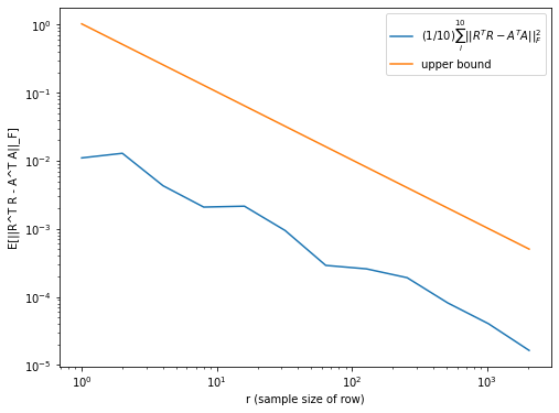
さらに,\(\mathbb{E}\left[ \lVert R^\top R - A^\top A \rVert_\mathrm{F}^2 \right] \le \frac{\lVert A \rVert_\mathrm{F}^4}{r}\)であることを確認します.具体的には,\(r\)を増やしてみて,誤差\(\lVert R^\top R - A^\top A \rVert_\mathrm{F}^2\)が減少することを見てみます.
[42]:
sample_size = 10

errors = []

rs = [2**k for k in range(12)]
for r in rs:
    mean = 0
    for _ in range(sample_size):
        row_indices = sample_rows(SQA, r)
        R = construct_R(SQA, A, row_indices)

        mean += np.linalg.norm(R.T @ R - A.T @ A)**2

    mean = mean/sample_size
    errors.append(mean)

    print(f"r={r}", mean, np.linalg.norm(A)**4/r)
r=1 0.011036088608588065 1.031494140624999
r=2 0.012900277652816452 0.5157470703124994
r=4 0.004301352915359831 0.2578735351562497
r=8 0.002086925152078077 0.12893676757812486
r=16 0.002153392048352806 0.06446838378906243
r=32 0.0009459364084887019 0.032234191894531215
r=64 0.0002901357148178583 0.016117095947265608
r=128 0.00025792208961707787 0.008058547973632804
r=256 0.00019129401249491832 0.004029273986816402
r=512 8.136658623254179e-05 0.002014636993408201
r=1024 4.0273416560124284e-05 0.0010073184967041005
r=2048 1.6310662494746377e-05 0.0005036592483520502
[43]:
plt.figure(figsize=(8, 6))
plt.plot(rs, errors, label="$(1/10)\sum_i^{10} || R^T R - A^T A ||_F^2$")
plt.plot(rs, [np.linalg.norm(A)**4/r for r in rs], label="upper bound")
plt.xlabel("r (sample size of row)")
plt.ylabel("E[||R^T R - A^T A||_F]")
plt.xscale("log")
plt.yscale("log")
plt.legend()
plt.show()
なお,関数construct_Rはただの確認用なので,実際には使われないことに注意してください.
[45]:
np.linalg.norm(R[0,:]), np.linalg.norm(R[1,:]), np.linalg.norm(A)/math.sqrt(r), np.linalg.norm(R), np.linalg.norm(A)
[45]:
(0.022269051271467524,
 0.022269051271467524,
 0.02226905127146753,
 1.0077822185373182,
 1.0077822185373184)
Step 2. 列のサンプリング:\(CC^\top \approx RR^\top\)を満たすような\(C\)を構成する.#
次に,Step2について実装します. ## 列添字をサンプルする関数の実装 Step 2の「等確率で\({0,1,\dots,r-1}\)から数字をサンプリングし結果を\(s\)とする.そして確率\(\frac{R_{s,j}^2}{\norm{R_{s,\ast}}^2} = \frac{A_{i_s,j}^2}{\norm{A_{i_s,\ast}}^2}\)で列添字をサンプリングし,結果を\(j_t\)とする.この操作を\(c\)回行い,サンプリングされた列添字を\(j_0,\dots,j_{c-1}\)とする」の部分について実装します.
[46]:
def sample_cols(SQA, row_indices, c):
    r = len(row_indices)
    col_indices = []
    for t in range(c):
        s   = np.random.randint(r)
        i_s = row_indices[s]
        j_t = SQA.sample2(i_s)
        col_indices.append(j_t)

    return col_indices
[48]:
r = 10
row_indices = sample_rows(SQA, r)

c = 20
col_indices = sample_cols(SQA, row_indices, c)

print("サンプルされた列添字:\n[j_0, i_1, ..., j_c-1] = ", col_indices)
サンプルされた列添字:
[j_0, i_1, ..., j_c-1] =  [12, 290, 76, 146, 2, 287, 150, 48, 182, 114, 182, 194, 122, 247, 243, 47, 76, 41, 198, 206]
\(r \times c\)の行列\(C\)を構成する関数の実装#
Step2の「\(r \times c\)の行列\(C\)を第\(t\)列が \(\frac{\norm{R}_\mathrm{F}}{\sqrt{c}} \frac{R_{\ast,j_t}}{\norm{R_{\ast,j_t}}} = \frac{\norm{A}_\mathrm{F}}{\sqrt{c}} \frac{R_{\ast,j_t}}{\norm{R_{\ast,j_t}}}\)」となるように構成する」という部分について実装します. \(R_{\ast,j_t}\)について注目します.行列\(R\)の\(s\)行目は\(\frac{\norm{A}_\mathrm{F}}{\sqrt{r}} \frac{A_{i_s,\ast}}{\norm{A_{i_s,\ast}}}\)であるので, 行列\(R\)の第\(j_t\)列\(R_{\ast,j_t}\)は
となります.このことを踏まえると,行列\(C\)を構成する関数は次のようになります.
[49]:
def construct_C(SQA, row_indices, col_indices):
    normAF = SQA.normF()
    r, c = len(row_indices), len(col_indices)

    # 行列Cを構成する
    C = np.zeros((r, c))
    for t in range(c):

        # Rのj_t列を構成する
        R_jt = np.zeros(r)
        j_t = col_indices[t]
        for s in range(r):
            i_s = row_indices[s]
            R_jt[s] = (normAF/(math.sqrt(r) * SQA.norm(i_s))) * SQA.query(i_s, j_t)

        # Cのt列を構成
        C[:, t] = (normAF/math.sqrt(c)) * R_jt/np.linalg.norm(R_jt)

    return C
\(CC^\top \approx RR^\top\)の確認#
\(CC^\top \approx RR^\top\)であることを前述と時と同様にして確認してみます.
[56]:
r, c = 10, 20
[57]:
row_indices = sample_rows(SQA, r)
col_indices = sample_cols(SQA, row_indices, c)

R = construct_R(SQA, A, row_indices)
C = construct_C(SQA, row_indices, col_indices)

error = np.linalg.norm(R @ R.T - C @ C.T)
print("誤差", error)
誤差 0.12079629623014908
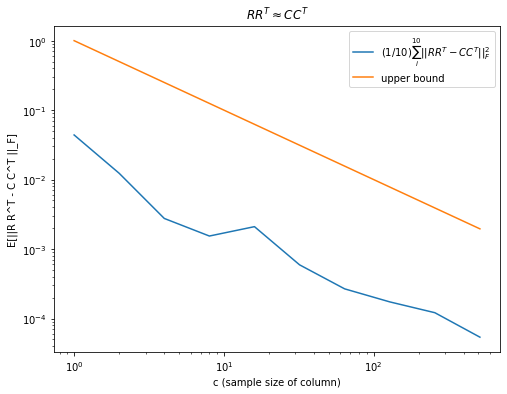
\(\mathbb{E}\left[ \lVert RR^\top - AA^\top \rVert_\mathrm{F}^2 \right] \le \frac{\lVert R \rVert_\mathrm{F}^4}{c}\)であることを確認します.具体的には,\(c\)を増やしてみて,誤差\(\lVert RR^\top - AA^\top \rVert_\mathrm{F}^2\)が減少することを見てみます.
[58]:
sample_size = 10

# E(R R.T) = C C.Tを確認する

# Rを作る
r = 10
row_indices = sample_rows(SQA, r)
R = construct_R(SQA, A, row_indices)

cs = [2**i for i in range(10)]

errors = []
for c in cs:
    mean = 0
    for _ in range(sample_size):
        # Cを作る
        col_indices = sample_cols(SQA, row_indices, c)
        C = construct_C(SQA, row_indices, col_indices)

        mean += np.linalg.norm(R @ R.T - C @ C.T)**2

    mean = mean/sample_size
    errors.append(mean)

    print(f"c={c}", mean, np.linalg.norm(R)**4/c)
c=1 0.0439018565995124 1.0314941406249971
c=2 0.01231327307140965 0.5157470703124986
c=4 0.0027570746630107973 0.2578735351562493
c=8 0.0015392452097097507 0.12893676757812464
c=16 0.002100567090502002 0.06446838378906232
c=32 0.0005925130682599771 0.03223419189453116
c=64 0.00026716441867974096 0.01611709594726558
c=128 0.00017349561289635792 0.00805854797363279
c=256 0.0001212114849485813 0.004029273986816395
c=512 5.384591647598512e-05 0.0020146369934081975
[59]:
plt.figure(figsize=(8, 6))
plt.plot(cs, errors, label="$(1/10)\sum_i^{10} || RR^T - CC^T ||_F^2$")
plt.plot(cs, [1/c for c in cs], label="upper bound")
plt.xlabel("c (sample size of column)")
plt.ylabel("E[||R R^T - C C^T ||_F]")
plt.xscale("log")
plt.yscale("log")
plt.title(r"$RR^T\approx CC^T$")
plt.legend()
plt.show()
Step 3:特異値分解#
最後に,Step3について考えます.Step3は行列\(C\)を特異値分解をするだけなのであり,この部分はNumPyの関数を使います .
[62]:
def qi_svd(SQA, r, c):

    # Step 1
    row_indices = sample_rows(SQA, r)

    # Step 2
    col_indices = sample_cols(SQA, row_indices, c)
    C = construct_C(SQA, row_indices, col_indices)

    # Step 3
    W, S, _ = np.linalg.svd(C)

    return row_indices, W, S

r, c = 100, 100
row_indices, W, S = qi_svd(SQA, r, c)
print("{i_0,...i_r-1} = \n", row_indices)
print("left singular vector of C =\n", W)
print("singular values of C =\n", S)
{i_0,...i_r-1} =
 [79, 131, 236, 138, 78, 41, 85, 354, 123, 169, 337, 258, 140, 76, 150, 308, 235, 238, 96, 231, 138, 258, 308, 211, 254, 260, 36, 307, 199, 195, 186, 124, 305, 85, 227, 323, 8, 129, 383, 8, 246, 132, 59, 145, 84, 129, 80, 129, 316, 95, 30, 11, 1, 211, 155, 271, 129, 106, 30, 5, 155, 256, 367, 266, 304, 182, 146, 195, 194, 55, 314, 4, 109, 186, 383, 220, 199, 220, 371, 159, 238, 153, 354, 289, 132, 314, 304, 181, 68, 55, 333, 229, 143, 231, 168, 35, 234, 137, 137, 79]
left singular vector of C =
 [[-0.10078665  0.05567284  0.32115091 ... -0.00234017  0.00356132
   0.93119914]
 [-0.09960004 -0.07489795  0.1081485  ... -0.01584392  0.02411162
  -0.04766102]
 [-0.09953486 -0.07910364 -0.05188662 ...  0.00095203 -0.00144882
   0.01363859]
 ...
 [-0.09931901 -0.09232038 -0.08066682 ... -0.09563616  0.14554116
   0.03532856]
 [-0.09931901 -0.09232038 -0.08066682 ...  0.08259732 -0.12569838
   0.03532856]
 [-0.10078665  0.05567284  0.05176083 ... -0.02035416  0.03097539
  -0.0232938 ]]
singular values of C =
 [1.00242849e+00 1.03740617e-01 9.87669694e-17 9.87669694e-17
 9.87669694e-17 9.87669694e-17 9.87669694e-17 9.87669694e-17
 9.87669694e-17 9.87669694e-17 9.87669694e-17 9.87669694e-17
 9.87669694e-17 9.87669694e-17 9.87669694e-17 9.87669694e-17
 9.87669694e-17 9.87669694e-17 9.87669694e-17 9.87669694e-17
 9.87669694e-17 9.87669694e-17 9.87669694e-17 9.87669694e-17
 9.87669694e-17 9.87669694e-17 9.87669694e-17 9.87669694e-17
 9.87669694e-17 9.87669694e-17 9.87669694e-17 9.87669694e-17
 9.87669694e-17 9.87669694e-17 9.87669694e-17 9.87669694e-17
 9.87669694e-17 9.87669694e-17 9.87669694e-17 9.87669694e-17
 9.87669694e-17 9.87669694e-17 9.87669694e-17 9.87669694e-17
 9.87669694e-17 9.87669694e-17 9.87669694e-17 9.87669694e-17
 9.87669694e-17 9.87669694e-17 9.87669694e-17 9.87669694e-17
 9.87669694e-17 9.87669694e-17 9.87669694e-17 9.87669694e-17
 9.87669694e-17 9.87669694e-17 9.87669694e-17 9.87669694e-17
 9.87669694e-17 9.87669694e-17 9.87669694e-17 9.87669694e-17
 9.87669694e-17 9.87669694e-17 9.87669694e-17 9.87669694e-17
 9.87669694e-17 9.87669694e-17 9.87669694e-17 9.87669694e-17
 9.87669694e-17 9.87669694e-17 9.87669694e-17 9.87669694e-17
 9.87669694e-17 9.87669694e-17 9.87669694e-17 9.87669694e-17
 9.87669694e-17 9.87669694e-17 9.87669694e-17 9.87669694e-17
 9.87669694e-17 9.87669694e-17 9.87669694e-17 9.87669694e-17
 9.87669694e-17 9.87669694e-17 9.87669694e-17 9.87669694e-17
 9.87669694e-17 9.87669694e-17 9.87669694e-17 9.87669694e-17
 9.87669694e-17 9.87669694e-17 9.87669694e-17 3.00449313e-17]
\(C\)の特異値・特異ベクトルと\(A\)の特異値・特異ベクトルについて#
特異値について#
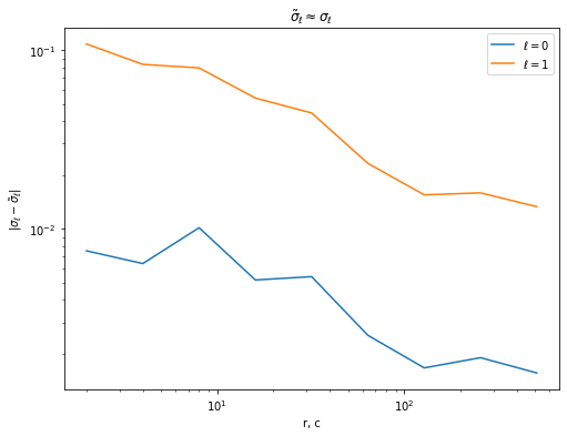
上記のアルゴリズムで得られた\(C\)の特異値\(\tilde{\sigma}_\ell\)(S)が,行列\(A\)の特異値\(\sigma_\ell\)(exact_S)を近似していることを見てみます.
[63]:
r, c = 20, 20
_, _, S = qi_svd(SQA, r, c)
print(f"{m}x{n}の行列Aの特異値: \n", exact_S)
print(f"\n{r}x{c}の行列Cの特異値: \n", S)
400x300の行列Aの特異値:
 [1.00000000e+00 1.25000000e-01 5.19213094e-16 4.79345167e-16
 4.71732210e-16 4.58242570e-16 4.18376202e-16 3.81834821e-16
 3.51484432e-16 3.47825823e-16 3.15975052e-16 3.06894888e-16
 2.92151597e-16 2.76922056e-16 2.60478793e-16 2.58559675e-16
 2.32224610e-16 2.30232802e-16 2.14765425e-16 2.08972139e-16
 2.02095864e-16 1.59139236e-16 1.54982739e-16 1.45129604e-16
 1.28041119e-16 1.23098986e-16 1.21378664e-16 9.86021132e-17
 9.71529166e-17 9.71529166e-17 9.71529166e-17 9.71529166e-17
 9.71529166e-17 9.71529166e-17 9.71529166e-17 9.71529166e-17
 9.71529166e-17 9.71529166e-17 9.71529166e-17 9.71529166e-17
 9.71529166e-17 9.71529166e-17 9.71529166e-17 9.71529166e-17
 9.71529166e-17 9.71529166e-17 9.71529166e-17 9.71529166e-17
 9.71529166e-17 9.71529166e-17 9.71529166e-17 9.71529166e-17
 9.71529166e-17 9.71529166e-17 9.71529166e-17 9.71529166e-17
 9.71529166e-17 9.71529166e-17 9.71529166e-17 9.71529166e-17
 9.71529166e-17 9.71529166e-17 9.71529166e-17 9.71529166e-17
 9.71529166e-17 9.71529166e-17 9.71529166e-17 9.71529166e-17
 9.71529166e-17 9.71529166e-17 9.71529166e-17 9.71529166e-17
 9.71529166e-17 9.71529166e-17 9.71529166e-17 9.71529166e-17
 9.71529166e-17 9.71529166e-17 9.71529166e-17 9.71529166e-17
 9.71529166e-17 9.71529166e-17 9.71529166e-17 9.71529166e-17
 9.71529166e-17 9.71529166e-17 9.71529166e-17 9.71529166e-17
 9.71529166e-17 9.71529166e-17 9.71529166e-17 9.71529166e-17
 9.71529166e-17 9.71529166e-17 9.71529166e-17 9.71529166e-17
 9.71529166e-17 9.71529166e-17 9.71529166e-17 9.71529166e-17
 9.71529166e-17 9.71529166e-17 9.71529166e-17 9.71529166e-17
 9.71529166e-17 9.71529166e-17 9.71529166e-17 9.71529166e-17
 9.71529166e-17 9.71529166e-17 9.71529166e-17 9.71529166e-17
 9.71529166e-17 9.71529166e-17 9.71529166e-17 9.71529166e-17
 9.71529166e-17 9.71529166e-17 9.71529166e-17 9.71529166e-17
 9.71529166e-17 9.71529166e-17 9.71529166e-17 9.71529166e-17
 9.71529166e-17 9.71529166e-17 9.71529166e-17 9.71529166e-17
 9.71529166e-17 9.71529166e-17 9.71529166e-17 9.71529166e-17
 9.71529166e-17 9.71529166e-17 9.71529166e-17 9.71529166e-17
 9.71529166e-17 9.71529166e-17 9.71529166e-17 9.71529166e-17
 9.71529166e-17 9.71529166e-17 9.71529166e-17 9.71529166e-17
 9.71529166e-17 9.71529166e-17 9.71529166e-17 9.71529166e-17
 9.71529166e-17 9.71529166e-17 9.71529166e-17 9.71529166e-17
 9.71529166e-17 9.71529166e-17 9.71529166e-17 9.71529166e-17
 9.71529166e-17 9.71529166e-17 9.71529166e-17 9.71529166e-17
 9.71529166e-17 9.71529166e-17 9.71529166e-17 9.71529166e-17
 9.71529166e-17 9.71529166e-17 9.71529166e-17 9.71529166e-17
 9.71529166e-17 9.71529166e-17 9.71529166e-17 9.71529166e-17
 9.71529166e-17 9.71529166e-17 9.71529166e-17 9.71529166e-17
 9.71529166e-17 9.71529166e-17 9.71529166e-17 9.71529166e-17
 9.71529166e-17 9.71529166e-17 9.71529166e-17 9.71529166e-17
 9.71529166e-17 9.71529166e-17 9.71529166e-17 9.71529166e-17
 9.71529166e-17 9.71529166e-17 9.71529166e-17 9.71529166e-17
 9.71529166e-17 9.71529166e-17 9.71529166e-17 9.71529166e-17
 9.71529166e-17 9.71529166e-17 9.71529166e-17 9.71529166e-17
 9.71529166e-17 9.71529166e-17 9.71529166e-17 9.71529166e-17
 9.71529166e-17 9.71529166e-17 9.71529166e-17 9.71529166e-17
 9.71529166e-17 9.71529166e-17 9.71529166e-17 9.71529166e-17
 9.71529166e-17 9.71529166e-17 9.71529166e-17 9.71529166e-17
 9.71529166e-17 9.71529166e-17 9.71529166e-17 9.71529166e-17
 9.71529166e-17 9.71529166e-17 9.71529166e-17 9.71529166e-17
 9.71529166e-17 9.71529166e-17 9.71529166e-17 9.71529166e-17
 9.71529166e-17 9.71529166e-17 9.71529166e-17 9.71529166e-17
 9.71529166e-17 9.71529166e-17 9.71529166e-17 9.71529166e-17
 9.71529166e-17 9.71529166e-17 9.71529166e-17 9.71529166e-17
 9.71529166e-17 9.71529166e-17 9.71529166e-17 9.71529166e-17
 9.71529166e-17 9.71529166e-17 9.71529166e-17 9.71529166e-17
 9.71529166e-17 9.71529166e-17 9.71529166e-17 9.71529166e-17
 9.71529166e-17 9.71529166e-17 9.71529166e-17 9.71529166e-17
 9.71529166e-17 9.71529166e-17 9.71529166e-17 9.71529166e-17
 9.71529166e-17 9.71529166e-17 9.71529166e-17 9.71529166e-17
 9.71529166e-17 9.71529166e-17 9.71529166e-17 9.71529166e-17
 9.71529166e-17 9.71529166e-17 9.71529166e-17 9.71529166e-17
 9.71529166e-17 9.71529166e-17 9.71529166e-17 9.71529166e-17
 9.71529166e-17 9.71529166e-17 9.71529166e-17 9.71529166e-17
 9.71529166e-17 9.71529166e-17 9.71529166e-17 9.71529166e-17
 9.71529166e-17 9.71529166e-17 9.71529166e-17 9.71529166e-17
 9.71529166e-17 9.71529166e-17 9.71529166e-17 9.71529166e-17
 9.71529166e-17 8.78031527e-17 6.59778865e-17 5.63605870e-17
 4.49028869e-17 2.86026833e-17 1.75002194e-17 3.56813390e-18]

20x20の行列Cの特異値:
 [1.00490103e+00 7.61506021e-02 1.21927212e-16 4.18890547e-17
 3.72992896e-17 3.63914528e-17 2.97914887e-17 2.87506791e-17
 2.44828993e-17 2.13046125e-17 1.99266041e-17 1.53090350e-17
 1.33693534e-17 9.03175877e-18 8.53422448e-18 5.09049230e-18
 3.77324832e-18 2.06136031e-18 1.41230911e-33 6.38038974e-34]
サンプル数\(r,c\)を増やしたときの特異値に関する誤差についてみてみます.行列\(A\)のランク分だけ\(C\)の特異値に注目します.
[66]:
sample_size = 10

rs = [2**i for i in range(1, 10)]
cs = [2**i for i in range(1, 10)]

hist0 = []
hist1 = []
for r, c in zip(rs, cs):
    mean0 = 0
    mean1 = 0
    for _ in range(sample_size):
        _, _, S = qi_svd(SQA, r, c)
        mean0 += abs(S[0] - exact_S[0])
        mean1 += abs(S[1] - exact_S[1])

    mean0 = mean0/sample_size
    mean1 = mean1/sample_size
    hist0.append(mean0)
    hist1.append(mean1)

    print(f"(r,c)=({r},{c}):", mean0, mean1)
(r,c)=(2,2): 0.007605164936364128 0.10077677401493898
(r,c)=(4,4): 0.006664163493095154 0.08303654467706957
(r,c)=(8,8): 0.011376142261109523 0.07973403408947627
(r,c)=(16,16): 0.009745271459953176 0.06004110776570289
(r,c)=(32,32): 0.003609230642555905 0.031184591754424763
(r,c)=(64,64): 0.004273053488123823 0.03890602246205678
(r,c)=(128,128): 0.002837380586722571 0.024082138257608424
(r,c)=(256,256): 0.00208143073207121 0.018202510064449937
(r,c)=(512,512): 0.0017952579212976772 0.014526341778711576
[65]:
plt.figure(figsize=(8, 6))
plt.plot(rs, hist0, label=r"$\ell=0$")
plt.plot(rs, hist1, label=r"$\ell=1$")
plt.xscale("log")
plt.yscale("log")
plt.xlabel("r, c")
plt.ylabel(r"$|\sigma_\ell - \tilde{\sigma}_\ell|$")
plt.title(r"$\tilde{\sigma}_\ell \approx \sigma_\ell$")
plt.legend()
plt.show()
なお,サンプル数\(r,c\)が行列\(A\)のサイズよりも小さい場合,\(C\)のサイズは\(A\)のサイズよりも小さくなります.そのため,\(A\)の特異値をそのまま計算するよりも,高速に近似特異値を得ることが期待できます.(\(\mathrm{SQ}(A)\)の構築時間を含めれると,遅くなることに注意)
[74]:
import time

start_time = time.time()
exact_S = sp.linalg.svdvals(A)
print("SciPyの特異値計算の時間\n", time.time() - start_time)

start_time = time.time()
# SQA = MatrixBasedDataStructure(A) # SQ(A)の構築も含めると遅くなる
_, _, S = qi_svd(SQA, 10, 10)
print("qi_svdを用いた時の特異値計算の時間\n", time.time() - start_time)

print("特異値の誤差", np.abs(exact_S[:2] - S[:2]))
SciPyの特異値計算の時間
 0.017342090606689453
qi_svdを用いた時の特異値計算の時間
 0.0013911724090576172
特異値の誤差 [0.00457841 0.04470537]
右特異ベクトルについて#
行列\(A\)の右特異ベクトル\(v^{(\ell)}\)は,
のようにして近似されます.このことを確認してみましょう.
[75]:
r, c = 100, 100
row_indices, W, S = qi_svd(SQA, r, c)

R = construct_R(SQA, A, row_indices)
[76]:
v0 = R.T @ W[:,0] / S[0]

print("0番目の特異値に対応するAの右特異ベクトル")
print("近似:\n",   v0)
print("SciPy:\n", exact_V[:,0])
0番目の特異値に対応するAの右特異ベクトル
近似:
 [-0.0317202   0.01337399 -0.11415716  0.06198199 -0.05629502 -0.03856402
  0.07927241 -0.05296198  0.02053256  0.07143687 -0.06066683  0.06599246
  0.08793431 -0.05312667  0.051438   -0.01644564 -0.05498971  0.03757013
 -0.00098816  0.02539686  0.06564687 -0.00855814 -0.0259037  -0.05998523
  0.05305378  0.08943291  0.07003928  0.00999123  0.04687588  0.00265625
 -0.09704059  0.07938635 -0.01840886  0.06111095 -0.06052255 -0.07395583
 -0.0521981   0.11650144 -0.09268968  0.07901958  0.02008417  0.08155085
 -0.04346777  0.01810488  0.03339253  0.05137885 -0.03231164  0.03518399
 -0.03111885  0.03459961  0.00977295  0.03586271 -0.10363354 -0.07319737
 -0.0802782   0.03757656  0.02940295 -0.02734621 -0.03605049 -0.0772996
  0.05253919 -0.06384619  0.01248809  0.00919471  0.08133145 -0.07976466
  0.07494208 -0.08056276 -0.07593681  0.02836961  0.04319938  0.03126609
  0.033294    0.1033259  -0.07034601  0.10302226 -0.09485786  0.08655116
  0.0194916   0.01596536 -0.0566828   0.08449272  0.02083656  0.08549993
 -0.00218206  0.00948511  0.02293383 -0.01769414 -0.07367503  0.00033869
 -0.04419602  0.10288678 -0.06686099  0.04419152  0.01094282 -0.01183871
  0.05867622 -0.02852445 -0.10442126  0.00174744 -0.01631248  0.05210681
 -0.01571766 -0.02589921 -0.08469993 -0.07157025 -0.0230451  -0.06465406
  0.00617937 -0.0159394   0.07770179 -0.02575547 -0.07170193 -0.06723837
 -0.04396394  0.03729801 -0.00641077 -0.07978389 -0.05345854  0.02760726
 -0.02578446  0.00591991  0.08548548  0.02656586  0.13203495 -0.03676117
 -0.06378039 -0.01779187 -0.09531531  0.02193487 -0.09872355 -0.00112499
  0.01478052  0.03016424 -0.03330164 -0.04999261  0.04666671 -0.0789648
  0.04571095 -0.0003321  -0.05986715 -0.00819154 -0.05777269 -0.05001009
  0.06926649 -0.02717667 -0.11020916  0.06314345  0.04643599 -0.01661893
 -0.03868591 -0.08211097  0.05058854 -0.05164187  0.01467088 -0.04339066
 -0.01783837  0.08601976 -0.1095638   0.0054588  -0.00342149 -0.09726745
 -0.03630337  0.02420097 -0.05219577 -0.06499896 -0.0011301  -0.01747065
  0.04274382 -0.04308753  0.05683675  0.0512726  -0.01191697  0.03852084
  0.08130772  0.03795078 -0.01944249  0.03060062  0.0523495   0.02011647
 -0.0880724  -0.05803288 -0.11355218 -0.00479497  0.0039829  -0.07985159
 -0.01587512 -0.03129549 -0.03690483 -0.02547485 -0.04708811 -0.017056
  0.01738491  0.00883852 -0.1573275  -0.06953934 -0.04309797 -0.08133134
 -0.06846626 -0.00274993  0.0155446   0.05527531  0.00888762 -0.08007245
  0.02708738 -0.00783943  0.09025781  0.02962462  0.15465978  0.05453309
  0.05973076 -0.03082224  0.00290697  0.08462897 -0.08427127  0.13412481
 -0.04548615  0.04383659 -0.01316888 -0.00543999  0.0320396   0.05633077
 -0.04379285  0.11285006 -0.01666589  0.10728228  0.00355295 -0.02455303
  0.06540515 -0.00571469 -0.14216609 -0.02847352  0.0749826   0.01440262
  0.00832115 -0.03356875  0.07404006  0.04974037  0.05205633  0.0340721
  0.0260405   0.00697726  0.01628316  0.05733054  0.05572234 -0.01441417
 -0.09585749 -0.0509137  -0.03943181 -0.03281695  0.04084048  0.15735757
 -0.00024769 -0.1315968  -0.01233281 -0.01006828  0.02565003  0.03327864
 -0.05773076  0.02379497 -0.03868227 -0.02009777  0.02232155  0.02321261
  0.11474818 -0.01715254  0.00643562  0.07770879  0.00178848  0.02780374
  0.06755107  0.01103524 -0.0750486  -0.00611766  0.01811955 -0.04082593
  0.02820813 -0.04598371 -0.0077759   0.10142964  0.09072496 -0.01452512
  0.0361294  -0.00788169  0.04839007  0.04639304 -0.02924079 -0.09581713
  0.05989333 -0.00654495  0.09971479  0.06922174 -0.02830517 -0.01349306
 -0.06510445  0.01003437  0.07008415  0.06489023  0.0167468  -0.01076254]
SciPy:
 [-0.03178579  0.01339787 -0.1143845   0.06210105 -0.05640416 -0.03864014
  0.07942287 -0.05306616  0.0205774   0.0715718  -0.06078328  0.06612246
  0.08810335 -0.05323437  0.05153945 -0.01648487 -0.05510182  0.03764083
 -0.00099093  0.02545148  0.06577178 -0.00858007 -0.02595692 -0.0601031
  0.0531583   0.08960578  0.0701723   0.01000783  0.04696291  0.0026565
 -0.09723311  0.07954568 -0.01844061  0.06122542 -0.06063984 -0.07410657
 -0.05229871  0.11672668 -0.09286865  0.07917701  0.02012488  0.08171221
 -0.04355533  0.01813954  0.03345575  0.0514816  -0.03237935  0.03525824
 -0.03117853  0.03466819  0.00978781  0.03593037 -0.10383397 -0.07333392
 -0.08043726  0.0376514   0.0294628  -0.02740079 -0.03612539 -0.07744662
  0.052643   -0.06397362  0.01251978  0.00921097  0.08149118 -0.07992301
  0.07509322 -0.08071959 -0.07609187  0.02842743  0.04328069  0.03132377
  0.03336238  0.10352992 -0.07048071  0.10322216 -0.09504197  0.08671549
  0.01952856  0.01599235 -0.0567889   0.08465883  0.02087572  0.08566471
 -0.00219     0.00950963  0.02298541 -0.01772501 -0.07381223  0.00033611
 -0.04427933  0.1030884  -0.0669901   0.04427171  0.01096017 -0.01186036
  0.05879242 -0.02858395 -0.10463549  0.00175337 -0.01635007  0.05220833
 -0.01574671 -0.02594836 -0.08486516 -0.07170336 -0.02309082 -0.0647826
  0.00618636 -0.01597017  0.07785602 -0.02580621 -0.07183828 -0.06737655
 -0.04404622  0.03736789 -0.00642312 -0.07994316 -0.05355942  0.02766029
 -0.02584077  0.00592402  0.08565684  0.02661693  0.13228927 -0.03683485
 -0.06389875 -0.01782499 -0.09549502  0.02198091 -0.09891416 -0.00112374
  0.01481104  0.0302231  -0.03336965 -0.05009244  0.04676617 -0.07912072
  0.04579826 -0.00032691 -0.05997921 -0.00820417 -0.05788193 -0.05011023
  0.06939673 -0.02723142 -0.11042606  0.06326595  0.04652422 -0.01664543
 -0.03876942 -0.0822678   0.05067961 -0.05173948  0.01470153 -0.04348097
 -0.01787777  0.0861799  -0.10977688  0.00547187 -0.00343178 -0.09745301
 -0.03637709  0.02425079 -0.05229407 -0.06512647 -0.00113412 -0.01750239
  0.04283423 -0.04316742  0.05694969  0.05137446 -0.0119413   0.03859628
  0.08146537  0.03802787 -0.01947816  0.03066369  0.0524491   0.02014959
 -0.08824002 -0.05813942 -0.1137716  -0.0047998   0.0039882  -0.08001098
 -0.01590691 -0.03135636 -0.0369706  -0.02552279 -0.04717569 -0.01708627
  0.01741501  0.00885184 -0.15763194 -0.0696734  -0.04318288 -0.08148692
 -0.06860291 -0.00275695  0.01557192  0.05538071  0.00890811 -0.08022934
  0.02714474 -0.00785599  0.09043169  0.02968092  0.15496412  0.05464191
  0.05984439 -0.03088542  0.00291311  0.08479313 -0.08443903  0.13438914
 -0.04557197  0.04391762 -0.01319775 -0.0054477   0.03210176  0.05644166
 -0.04387738  0.11307303 -0.01669799  0.10748609  0.00356494 -0.02459806
  0.06553224 -0.00573285 -0.14244482 -0.02852883  0.07513035  0.0144233
  0.00833655 -0.0336364   0.07418805  0.04983916  0.05215753  0.03414352
  0.02609588  0.00699501  0.01631814  0.05744169  0.05582713 -0.01443581
 -0.09604381 -0.05101221 -0.03951222 -0.03287923  0.04091922  0.15766364
 -0.00024434 -0.13185333 -0.01236108 -0.01008769  0.02570283  0.03334367
 -0.05784436  0.02384133 -0.03875717 -0.02013642  0.02236463  0.02325399
  0.11496818 -0.01718518  0.00644599  0.07786043  0.00178812  0.02785964
  0.06768607  0.01104995 -0.07519349 -0.00612426  0.01815661 -0.04090824
  0.02826305 -0.04607949 -0.00779054  0.10163116  0.09090134 -0.01455158
  0.0361944  -0.007898    0.04848326  0.04648396 -0.02929724 -0.09599888
  0.06001497 -0.00655647  0.09990745  0.06935388 -0.02836367 -0.01351696
 -0.06524075  0.01004781  0.07021831  0.06501476  0.01677325 -0.01077529]
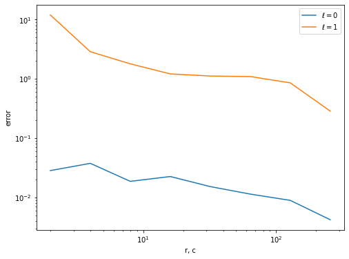
サンプル数を増やしていくにつれて,\(\norm{v^{(\ell)} - \tilde{v}^{(\ell)}}\)が小さくなることを確認します.
[79]:
errors = []
sample_size = 10
k = 0 # 確認する特異ベクトルの番号.
rs = [2**i for i in range(1, 9)]
cs = [2**i for i in range(1, 9)]

hist0 = []
hist1 = []

for r, c in zip(rs, cs):

    mean0 = 0
    mean1 = 0
    for _ in range(sample_size):
        row_indices, W, S = qi_svd(SQA, r, c)

        # 確認
        R = construct_R(SQA, A, row_indices)
        v0 = R.T @ W[:, 0]/S[0]
        v1 = R.T @ W[:, 1]/S[1]

        mean0 += np.linalg.norm(v0 - exact_V[:, 0])
        mean1 += np.linalg.norm(v1 - exact_V[:, 1])

    mean0 = mean0/sample_size
    mean1 = mean1/sample_size
    hist0.append(mean0)
    hist1.append(mean1)

    print(f"(r,c)=({r},{c}):", mean0, mean1, np.abs(S[:rankA] - exact_S[:rankA]))
(r,c)=(2,2): 0.02829504908539988 11.953080497719569 [0.05143816 0.21537544]
(r,c)=(4,4): 0.037495686271958616 2.864633876497967 [0.00751327 0.10171908]
(r,c)=(8,8): 0.018633988145829013 1.7889104770224038 [0.00145007 0.01220476]
(r,c)=(16,16): 0.02246828079147237 1.2119560370589524 [0.00659683 0.07613456]
(r,c)=(32,32): 0.015194689881244009 1.1144072028039513 [0.00340926 0.03121909]
(r,c)=(64,64): 0.011350414319032538 1.0925412277833169 [0.00151848 0.01160038]
(r,c)=(128,128): 0.008898171229586123 0.8549066952643022 [0.00144013 0.01211654]
(r,c)=(256,256): 0.0041891501005805205 0.28546587539012197 [3.09644045e-05 2.47466442e-04]
[81]:
plt.figure(figsize=(8, 6))
plt.plot(rs, hist0, label=r"$\ell=0$")
plt.plot(rs, hist1, label=r"$\ell=1$")
plt.xscale("log")
plt.yscale("log")
plt.xlabel("r, c")
plt.ylabel("error")
plt.title(r"")
plt.legend()
plt.show()
左特異ベクトルについて#
行列\(A\)の左特異ベクトル\(u^{(\ell)}\)は,
のようにして近似されます.このことを確認してみます.
[82]:
r, c = 1000, 1000
row_indices, W, S = qi_svd(SQA, r, c)
R = construct_R(SQA, A, row_indices)
[84]:
u0 = A @ R.T @ W[:,0] / (S[0]**2)

print("0番目の特異値に対応するAの左特異ベクトル")
print("近似:\n",   u0)
print("SciPy:\n", exact_U[:,0])
0番目の特異値に対応するAの左特異ベクトル
近似:
 [-0.0605458  -0.0704849  -0.07149567 -0.04855803 -0.06494327 -0.0608823
 -0.00690812 -0.04015194 -0.07384671 -0.0734254  -0.00876735 -0.05075763
 -0.05635925 -0.03699295 -0.03174713 -0.07583245 -0.00139154 -0.02593728
 -0.07389579 -0.04645488 -0.05951348 -0.03605792 -0.05254252 -0.01226802
 -0.00362969 -0.0339557  -0.04472962 -0.0125205  -0.07404588 -0.03484445
 -0.07841977 -0.08207029 -0.05855517 -0.06039629 -0.06840638 -0.06452022
 -0.06882283 -0.02948692 -0.06494297 -0.06989275 -0.00083706 -0.07390116
 -0.06036129 -0.05834352 -0.0173526  -0.05614958 -0.04937652 -0.03994919
 -0.01978992 -0.03851737 -0.03806637 -0.08059453 -0.02387455 -0.07240957
 -0.07010345 -0.08319091 -0.00675038 -0.01602705 -0.03474378 -0.02315195
 -0.05877738 -0.01669903 -0.04517126 -0.03589944 -0.00946414 -0.08191783
 -0.03327773 -0.07096757 -0.07956595 -0.07393915 -0.03677444 -0.05498509
 -0.00635478 -0.02331074 -0.0667158  -0.0048446  -0.05927138 -0.04358965
 -0.07173062 -0.07904759 -0.0728023  -0.04476247 -0.06216394 -0.05068522
 -0.07986796 -0.08303011 -0.03791738 -0.01840737 -0.03995369 -0.00265248
 -0.02539848 -0.02249231 -0.08164556 -0.04743769 -0.05679071 -0.05941819
 -0.0577563  -0.05288016 -0.00592677 -0.03649032 -0.00146731 -0.03588471
 -0.05995013 -0.01976901 -0.01166355 -0.04299707 -0.05190724 -0.029776
 -0.04378774 -0.0463587  -0.03521626 -0.05078906 -0.01696562 -0.01960544
 -0.07342023 -0.06143066 -0.05866729 -0.04179887 -0.08295138 -0.01211161
 -0.03385545 -0.08145    -0.0477917  -0.08235871 -0.070211   -0.03934347
 -0.01423589 -0.06718754 -0.02678061 -0.0756882  -0.07849846 -0.04628303
 -0.06796465 -0.01840771 -0.06584961 -0.03190238 -0.00906975 -0.06983423
 -0.05323478 -0.03375346 -0.04189315 -0.01298106 -0.03455251 -0.03931664
 -0.05917124 -0.07962125 -0.03689864 -0.01044661 -0.01134955 -0.0107187
 -0.06491777 -0.00575106 -0.00521567 -0.07257526 -0.01290219 -0.08276778
 -0.06561617 -0.07916155 -0.0674428  -0.03894268 -0.03202196 -0.02759434
 -0.0706788  -0.00872396 -0.03247791 -0.02014104 -0.00996913 -0.01419721
 -0.07869264 -0.06606762 -0.0274082  -0.00420174 -0.0122052  -0.05808773
 -0.05176395 -0.0566248  -0.00416218 -0.07744653 -0.06151638 -0.07639261
 -0.05347447 -0.06627271 -0.07669143 -0.03477293 -0.04141373 -0.03128679
 -0.03788901 -0.05323336 -0.08258669 -0.02300419 -0.002807   -0.00712448
 -0.00251053 -0.07134748 -0.05720149 -0.06478203 -0.05903397 -0.00977324
 -0.02724393 -0.05174461 -0.0596949  -0.06747449 -0.0706302  -0.05346121
 -0.02997381 -0.04722246 -0.04539428 -0.01989842 -0.05704522 -0.08253875
 -0.076835   -0.07251446 -0.07125862 -0.05001557 -0.00465223 -0.0815906
 -0.02634413 -0.08109756 -0.0491986  -0.03975387 -0.06204669 -0.02409887
 -0.01237883 -0.05061375 -0.07087539 -0.01549627 -0.04723927 -0.0798324
 -0.01603082 -0.04837712 -0.00276387 -0.05772191 -0.03471284 -0.00823026
 -0.01678352 -0.07274266 -0.03495152 -0.08061009 -0.07631995 -0.06716318
 -0.00873076 -0.06160927 -0.08070924 -0.04558438 -0.06143948 -0.07142257
 -0.056468   -0.03793588 -0.03122556 -0.05919834 -0.00885933 -0.0029276
 -0.0568097  -0.01650095 -0.06685359 -0.046717   -0.03655642 -0.03812575
 -0.04561245 -0.00911834 -0.08015103 -0.0662699  -0.04707998 -0.00862236
 -0.06604481 -0.0664349  -0.0580816  -0.05609323 -0.02730883 -0.02042405
 -0.01226267 -0.05435141 -0.06087473 -0.03697347 -0.00023972 -0.05346648
 -0.04716755 -0.02469469 -0.00302745 -0.03113723 -0.02623074 -0.02681332
 -0.05223701 -0.02821278 -0.0493041  -0.02786236 -0.02784349 -0.03131616
 -0.0546355  -0.06380391 -0.00023605 -0.05146422 -0.03066548 -0.05251106
 -0.07201202 -0.04256657 -0.02744108 -0.00875707 -0.02055682 -0.03793859
 -0.05096003 -0.02404277 -0.02215396 -0.04740809 -0.08059723 -0.08117378
 -0.04382467 -0.07713837 -0.08115339 -0.05283448 -0.04931161 -0.07286654
 -0.04332738 -0.03636768 -0.06870996 -0.02358293 -0.0416052  -0.08031554
 -0.0288785  -0.03039519 -0.00443046 -0.00799646 -0.03985718 -0.02861012
 -0.0356367  -0.01622956 -0.05600859 -0.00584186 -0.04529722 -0.0414683
 -0.00295963 -0.05200601 -0.03670453 -0.02870568 -0.03131672 -0.01109076
 -0.06158986 -0.05923834 -0.07795516 -0.07206882 -0.04505654 -0.08203382
 -0.04190346 -0.02162796 -0.03967774 -0.04925219 -0.04258829 -0.01581113
 -0.06189415 -0.02329364 -0.06518351 -0.0329322  -0.06291574 -0.0444857
 -0.07947668 -0.04571527 -0.06775138 -0.03454912 -0.01213915 -0.02988561
 -0.00573499 -0.04412681 -0.02397704 -0.01587559 -0.03690571 -0.01068382
 -0.01793798 -0.03995668 -0.00986041 -0.0808141  -0.00030202 -0.07198661
 -0.03742878 -0.03056998 -0.04473364 -0.02759723 -0.0140094  -0.01773207
 -0.04575469 -0.05951234 -0.05822442 -0.08182881 -0.06823165 -0.05164249
 -0.01971849 -0.03670303 -0.05498087 -0.07597282 -0.04423853 -0.01947815
 -0.06791941 -0.0294482  -0.01051621 -0.04196672 -0.02150881 -0.04872591
 -0.02877166 -0.06208905 -0.05471735 -0.05511436]
SciPy:
 [-0.06063178 -0.07056625 -0.07158246 -0.04862612 -0.06503195 -0.06095108
 -0.00693953 -0.04021985 -0.07394289 -0.07351338 -0.00878353 -0.05081582
 -0.05642742 -0.03704946 -0.0318087  -0.07593304 -0.00141568 -0.02599341
 -0.07399201 -0.04650953 -0.05959117 -0.03611226 -0.05260113 -0.01228628
 -0.00363698 -0.03401735 -0.04479451 -0.01254705 -0.0741346  -0.03491016
 -0.07853127 -0.08218143 -0.05863315 -0.06048798 -0.0684982  -0.06460986
 -0.06891866 -0.02954067 -0.06503005 -0.06997553 -0.00084306 -0.0740002
 -0.06045485 -0.05842809 -0.0173783  -0.05623333 -0.04943806 -0.04001221
 -0.01984121 -0.03857801 -0.03813133 -0.08068746 -0.02390982 -0.07250399
 -0.0702003  -0.08329509 -0.00678477 -0.01606309 -0.03480238 -0.02319961
 -0.058862   -0.01672736 -0.04524962 -0.03596486 -0.00950268 -0.08201297
 -0.03332387 -0.0710696  -0.07965349 -0.07402582 -0.03682144 -0.05505557
 -0.00636821 -0.02335395 -0.06680174 -0.00485834 -0.05936046 -0.04365236
 -0.0718282  -0.07914442 -0.07288395 -0.04483074 -0.06224089 -0.05074273
 -0.07996829 -0.08314655 -0.03797211 -0.01842989 -0.03999778 -0.00266692
 -0.02543578 -0.02253468 -0.08174462 -0.04750384 -0.05687514 -0.0594967
 -0.05783011 -0.0529424  -0.00593584 -0.03653522 -0.00148681 -0.03593123
 -0.06001967 -0.0198167  -0.01170331 -0.04304919 -0.05196441 -0.02982581
 -0.04385963 -0.04641885 -0.03527912 -0.05086332 -0.01700349 -0.01964498
 -0.07352595 -0.06151298 -0.05875747 -0.04185704 -0.08305182 -0.01212945
 -0.03391248 -0.08154055 -0.04785471 -0.0824541  -0.07031419 -0.03940017
 -0.01425221 -0.06726387 -0.02683388 -0.07579793 -0.07861089 -0.04634977
 -0.06804526 -0.01844644 -0.06593022 -0.03196295 -0.00909236 -0.06993697
 -0.05331092 -0.03380142 -0.0419535  -0.01300585 -0.03460886 -0.03936059
 -0.05925991 -0.07971551 -0.03694779 -0.01046141 -0.01136678 -0.01075114
 -0.0650068  -0.00576516 -0.00523565 -0.07265599 -0.01292018 -0.08285846
 -0.06568797 -0.07925332 -0.06752771 -0.03899369 -0.03206217 -0.0276371
 -0.07076888 -0.00874673 -0.03254125 -0.02016686 -0.00999661 -0.01424195
 -0.07878899 -0.06616008 -0.02745157 -0.00421571 -0.01222621 -0.0581739
 -0.05182444 -0.0567016  -0.00417239 -0.07753641 -0.0616052  -0.07648652
 -0.05355695 -0.06635803 -0.07679893 -0.0348233  -0.0414831  -0.03133529
 -0.0379397  -0.05329744 -0.08270502 -0.02303596 -0.00281382 -0.00715434
 -0.00251455 -0.07143812 -0.05728264 -0.06485961 -0.05912167 -0.00980228
 -0.02728896 -0.05180133 -0.05978358 -0.06756594 -0.07071727 -0.05354538
 -0.03002496 -0.04729218 -0.04545434 -0.01992118 -0.05712637 -0.08264747
 -0.07692423 -0.07261944 -0.07133902 -0.05009336 -0.0046716  -0.08170006
 -0.02638369 -0.08120615 -0.04926476 -0.03980993 -0.06211485 -0.02414838
 -0.01239285 -0.0506823  -0.07095273 -0.0155263  -0.0473167  -0.07994415
 -0.01606506 -0.04844704 -0.00277822 -0.05778958 -0.034761   -0.00826202
 -0.0168026  -0.07282904 -0.03500217 -0.08070908 -0.07642476 -0.0672386
 -0.008764   -0.06170246 -0.0808191  -0.04564182 -0.06153348 -0.0715151
 -0.0565438  -0.0379882  -0.03128069 -0.05928644 -0.0088728  -0.00293301
 -0.05688345 -0.01654686 -0.0669474  -0.04678061 -0.03661127 -0.03818637
 -0.04568726 -0.00915323 -0.08024214 -0.06635014 -0.04713686 -0.0086446
 -0.06612905 -0.06651602 -0.05814475 -0.05617944 -0.0273549  -0.02047405
 -0.01229146 -0.05442679 -0.06096082 -0.0370327  -0.00024619 -0.05353806
 -0.04724044 -0.02474614 -0.00303486 -0.03118458 -0.0262789  -0.02686085
 -0.05230675 -0.02825987 -0.04937317 -0.02789618 -0.02789151 -0.03135598
 -0.05471743 -0.0638749  -0.00026383 -0.05152938 -0.03071228 -0.05257198
 -0.07211434 -0.04264211 -0.0274817  -0.00878321 -0.0205986  -0.03799543
 -0.05102354 -0.02409885 -0.0221824  -0.04746076 -0.08069505 -0.08127258
 -0.04389224 -0.07722425 -0.08125058 -0.05289844 -0.04939296 -0.07295638
 -0.04337727 -0.03643595 -0.06880348 -0.02362328 -0.04167796 -0.08040976
 -0.02892012 -0.03043761 -0.0044412  -0.00802596 -0.03990368 -0.02864774
 -0.03569326 -0.01625035 -0.05607518 -0.00586505 -0.04537514 -0.04152883
 -0.00298864 -0.05208027 -0.03677207 -0.02873733 -0.03135558 -0.01111267
 -0.0616602  -0.0593312  -0.07805245 -0.07215897 -0.04512449 -0.0821318
 -0.04195338 -0.02165334 -0.03974893 -0.0493141  -0.04264729 -0.015829
 -0.06198071 -0.02332793 -0.06528109 -0.03297081 -0.06300878 -0.04453606
 -0.07958374 -0.04576957 -0.0678319  -0.03459215 -0.01216611 -0.02993966
 -0.00575253 -0.04419967 -0.0240268  -0.01591216 -0.03696948 -0.01070977
 -0.01797275 -0.04002642 -0.00989548 -0.0809272  -0.00032691 -0.07207141
 -0.03747797 -0.03060903 -0.04479431 -0.02763489 -0.01403073 -0.01775245
 -0.04581232 -0.05959357 -0.05831362 -0.08193596 -0.06832077 -0.05172321
 -0.01974377 -0.03675004 -0.05504588 -0.076076   -0.04428945 -0.01952937
 -0.06800251 -0.02949921 -0.01054801 -0.04201861 -0.02154635 -0.04880282
 -0.02883157 -0.06216436 -0.05477746 -0.05518749]
サンプル数を増やしていくにつれて,\(\norm{u^{(\ell)} - \tilde{u}^{(\ell)}}\)が小さくなることを確認します.
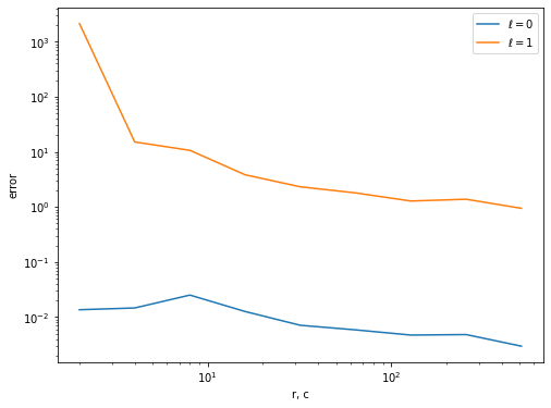
[85]:
sample_size = 20

hist0 = []
hist1 = []

rs = [2**i for i in range(1, 10)]
cs = [2**i for i in range(1, 10)]
for r, c in zip(rs, cs):

    mean0 = 0
    mean1 = 0
    for _ in range(sample_size):
        row_indices, W, S = qi_svd(SQA, r, c)

        # 確認
        R = construct_R(SQA, A, row_indices)
        u0 = A @ R.T @ W[:, 0]/S[0]**2
        u1 = A @ R.T @ W[:, 1]/S[1]**2
        mean0 += np.linalg.norm(u0 - exact_U[:, 0])
        mean1 += np.linalg.norm(u1 - exact_U[:, 1])

    mean0 = mean0/sample_size
    mean1 = mean1/sample_size
    hist0.append(mean0)
    hist1.append(mean1)

    print(f"(r,c)=({r},{c}):", mean0, mean1)
(r,c)=(2,2): 0.013603883719106055 2130.2608988385095
(r,c)=(4,4): 0.014645442873687764 15.121519302163557
(r,c)=(8,8): 0.02509946525614708 10.636265086191234
(r,c)=(16,16): 0.012625600458247736 3.8287808017213267
(r,c)=(32,32): 0.007096984858864107 2.3173803313471515
(r,c)=(64,64): 0.005862771726432317 1.7957413769009574
(r,c)=(128,128): 0.004717295673775422 1.279604646308625
(r,c)=(256,256): 0.004818623948890067 1.378776675271584
(r,c)=(512,512): 0.0029659244507325017 0.9435018957612348
[88]:
plt.figure(figsize=(8, 6))
plt.plot(rs, hist0, label=r"$\ell=0$")
plt.plot(rs, hist1, label=r"$\ell=1$")
plt.xscale("log")
plt.yscale("log")
plt.xlabel("r, c")
plt.ylabel("error")
plt.title(r"")
plt.legend()
plt.show()
まとめ#
量子インスパイアード古典アルゴリズムにおける,\(C\)の特異値分解までをみてきました.このノートブックでは,特異ベクトルの復元に,行列\(A\)や\(R\)と\(C\)の左特異ベクトルに関する行列-ベクトル積を行なっているため,元々の行列\(A\)の次元に関して多項式の計算量を必要とします.3_SQ(x).ipynbでは,このような計算量をかけずにSample, Query, Normそれぞれを実行することについて説明します.
参考文献#
András Gilyén, Seth Lloyd, and Ewin Tang, ‘’Quantum-inspired low-rank stochastic regression with logarithmic dependence on the dimension,’’ arXiv:1811.04909, (2018). https://arxiv.org/abs/1811.04909
Ewin Tang. 2019. A quantum-inspired classical algorithm for recommendation systems. In Proceedings of the 51st Annual ACM SIGACT Symposium on Theory of Computing (STOC 2019). Association for Computing Machinery, New York, NY, USA, 217–228. https://doi.org/10.1145/3313276.3316310
[ ]: